24.9 Vibrations

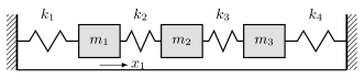
Chapter 13 §04 diagonalized two forms at once and then said, in one sentence, what the theorem was for: for a vibrating structure one matrix is the mass matrix, the other the stiffness matrix, the generalized eigenvalues are the squared natural frequencies, and the eigenvectors are the normal modes. This section turns that sentence into a theorem and reads off its consequences. Everything in it is linear algebra already proved, applied to one physical model; the model is the only new ingredient, and it is stated as a model, not derived.

Throughout, the field is $\mathbb{R}$ , and $n \ge 1$ is the number of moving masses.

A note on the letter $\mathbf{K}$ . In this section $\mathbf{K}$ is the stiffness matrix. Chapter 19 §09’s second-difference matrix always carries its size as a subscript, $\mathbf{K}_n$ , and it will appear below as exactly that; the two never collide.

24.9.1. A chain of masses and springs

Picture $n$ carts on a line, joined to each other and to two fixed walls by springs. Each cart is at rest in some position, and we track only its displacement from that position, so that the rest state is the zero vector. The question is what the system does when it is pushed and released.

Diagram. Labels: m_i, k_1, k_2, k_3, k_4, x_1

Two physical laws describe what happens, and both are assumptions, not theorems of this book. We give them a name and numbered clauses, so that the steps below can say which one they are using.

Definition 24.9.1 (The mass–spring model)

(P1) (Newton’s second law.) A mass $m_i > 0$ whose displacement is $x_i(t)$ obeys $m_i x_i''(t) = f_i(t)$ , where $f_i$ is the total force on it.
(P2) (Hooke’s law.) A spring of stiffness $k \ge 0$ whose two ends have moved by $a$ and $b$ pulls its ends together with force $k(b - a)$ acting on the end at $a$ , and $-k(b-a)$ on the end at $b$ . A wall is an end whose displacement is $0$ . A spring of stiffness $0$ exerts no force whatever, so it is the same thing as no spring at all.

Hooke’s law is an idealization: real springs obey it only for small displacements, and every real system also loses energy. We assume both laws exactly, and everything below is a theorem about that idealization; the energy loss reappears as the non-example below.

Take the chain in the picture: three masses $m_1, m_2, m_3$ and four springs $k_1, \dots, k_4$ , with $k_1$ joining the left wall to mass $1$ and $k_4$ joining mass $3$ to the right wall. The force on mass $1$ comes from the springs on either side of it, so by (P1) and (P2) of Definition 24.9.1, $\begin{aligned} m_1x_1'' &= -k_1x_1 + k_2(x_2 - x_1) , \\ m_2x_2'' &= -k_2(x_2 - x_1) + k_3(x_3 - x_2) , \\ m_3x_3'' &= -k_3(x_3 - x_2) - k_4x_3 . \end{aligned}$ Collecting the coefficients of $x_1, x_2, x_3$ on the right and moving the sign out front, this is $\mathbf{M}\mathbf{x}'' = -\mathbf{K}\mathbf{x}$ with $\mathbf{M} = \begin{pmatrix} m_1 & & \\ & m_2 & \\ & & m_3\end{pmatrix}, \quad \mathbf{K} = \begin{pmatrix} k_1 {+} k_2 & -k_2 & 0 \\ -k_2 & k_2 {+} k_3 & -k_3 \\ 0 & -k_3 & k_3 {+} k_4 \end{pmatrix} .$ The matrix $\mathbf{M}$ is diagonal with positive entries, hence positive definite. The matrix $\mathbf{K}$ is symmetric, and it is positive semidefinite for a reason worth isolating, so we record the general shape first.

A mass–spring system is a pair of forms: one that measures inertia and one that measures the price of a deformation.

Definition 24.9.2 (Mass–spring system)

A mass–spring system with $n$ degrees of freedom is a pair of real symmetric matrices $\mathbf{M}, \mathbf{K} \in M_n(\mathbb{R})$ with $\mathbf{M} \succ 0$ and $\mathbf{K} \succeq 0$ , called the mass matrix and the stiffness matrix. A motion of the system is a twice-differentiable function $\mathbf{x} \colon \mathbb{R} \to \mathbb{R}^n$ with

\mathbf{M}\mathbf{x}''(t) = -\mathbf{K}\mathbf{x}(t) \qquad \text{for every } t \in \mathbb{R} .

(24.9.1)

The same equation is read for a function $\mathbf{x} \colon \mathbb{R} \to \mathbb{C}^n$ whenever a complex trial solution is convenient; a motion without qualification is real.

In words: $\mathbf{M} \succ 0$ says every direction of motion costs some inertia, so no coordinate is massless; $\mathbf{K} \succeq 0$ says no deformation releases energy, so the rest state $\mathbf{x} = \mathbf{0}$ is not a hilltop. The quantities $\tfrac12(\mathbf{x}')^{\top}\mathbf{M}\mathbf{x}'$ and $\tfrac12\mathbf{x}^{\top}\mathbf{K}\mathbf{x}$ are what the model calls the kinetic and potential energy of the state $(\mathbf{x}, \mathbf{x}')$ — a third physical identification, on the same footing as (P1) and (P2) of Definition 24.9.1 and used nowhere in a proof — and the two definiteness hypotheses say exactly that the first is positive and the second non-negative away from rest.

For the chain, positive semidefiniteness of $\mathbf{K}$ is a factorization. Number the springs $1, \dots, n+1$ from left to right and let $\mathbf{B} \in M_{(n+1) \times n}(\mathbb{R})$ be the matrix whose row $e$ records how much spring $e$ is stretched: for the chain above, $\mathbf{B} = \begin{pmatrix} 1 & 0 & 0 \\ -1 & 1 & 0 \\ 0 & -1 & 1 \\ 0 & 0 & -1 \end{pmatrix}, \qquad \mathbf{K} = \mathbf{B}^{\top}\mathbf{D}_k\mathbf{B} ,$ where $\mathbf{D}_k = \operatorname{diag}(k_1, \dots, k_{n+1})$ . Multiplying out confirms the second identity entry by entry. Consequently $\mathbf{x}^{\top}\mathbf{K}\mathbf{x} = (\mathbf{B}\mathbf{x})^{\top}\mathbf{D}_k(\mathbf{B}\mathbf{x}) = \sum_{e} k_e\,(\mathbf{B}\mathbf{x})_e^2 \ \ge\ 0 ,$ a sum of squares weighted by the stiffnesses: the potential energy stored in the springs. Together with $\mathbf{K}^{\top} = \mathbf{K}$ this is Definition 13.1.1, so $\mathbf{K} \succeq 0$ with no computation of eigenvalues. (The matrix $\mathbf{B}$ is, up to a transpose and the deletion of the two wall rows, the incidence matrix of Chapter 3 §07, Definition 3.7.1, of the chain together with a choice of orientation for each spring: the orientation is what fixes the sign pattern of the rows, and it is what Definition 3.7.1 records as the head and the tail of an edge. The last section of this chapter takes that observation seriously.)

Three instances, simplest first.

Example (Three systems)

(a) $n = 1$ : one mass $m$ between two walls with springs $k_1, k_2$ . Then $\mathbf{M} = (m)$ and $\mathbf{K} = (k_1 + k_2)$ , both $1 \times 1$ .
(b) $n = 3$ with all masses equal to $m$ and all four stiffnesses equal to $k$ . Then $\mathbf{M} = m\mathbf{I}_3$ and $\mathbf{K} = k\mathbf{K}_3$ , where $\mathbf{K}_3$ is the second-difference matrix met in Proposition 19.9.6.
(c) The free chain: the same three masses joined to each other by $k_2, k_3$ but with no walls, so $k_1 = k_4 = 0$ . Then $\mathbf{K}$ is still symmetric and still $\mathbf{B}^{\top}\mathbf{D}_k\mathbf{B}$ , hence $\succeq 0$ , but now $\mathbf{K}\mathbf{1} = \mathbf{0}$ : sliding the whole chain sideways stretches nothing.

Case (c) is the degenerate one, and it is not a pathology to be excluded: it is why the definition asks only for $\mathbf{K} \succeq 0$ . A system with a direction of zero stiffness has a motion that is not a vibration at all, and the theorem below will produce it.

Change one clause and the definition stops describing this situation. If a cart also feels friction proportional to its velocity, the equation becomes $\mathbf{M}\mathbf{x}'' = -\mathbf{K}\mathbf{x} - \mathbf{C}\mathbf{x}'$ with $\mathbf{C} \succeq 0$ the damping matrix; the right-hand side is no longer a function of $\mathbf{x}$ alone, Eq. 24.9.1 fails, and the analysis of this section does not apply to it. The models differ in exactly one term, and everything below uses the absence of that term.

Warning. The natural frequencies are not the eigenvalues of $\mathbf{K}$ divided by the eigenvalues of $\mathbf{M}$ . Take $\mathbf{M} = \operatorname{diag}(1, 4)$ and $\mathbf{K} = \begin{psmallmatrix} 2 & -1 \\ -1 & 2\end{psmallmatrix}$ . The eigenvalues of $\mathbf{K}$ are $3$ and $1$ , those of $\mathbf{M}$ are $4$ and $1$ , so the four available quotients are $3, 3/4, 1$ and $1/4$ . The squared natural frequencies, computed from $\det(\mathbf{K} - \lambda\mathbf{M}) = 4\lambda^2 - 10\lambda + 3$ , are $\lambda = \tfrac{5 \pm \sqrt{13}}{4} \approx 2.151,\ 0.349 ,$ and neither is on the list. Mass and stiffness interact through their eigenvectors, not only through their eigenvalues; only when $\mathbf{M}$ is a scalar multiple of $\mathbf{I}$ does the naive rule hold.

24.9.2. Normal modes

A motion of one mass on one spring is a single oscillation. The hope is that a motion of $n$ masses is a superposition of $n$ such oscillations, each with its own frequency and its own shape. That hope is exactly Theorem 13.4.1, and the only thing needed before it is the one-dimensional case.

Lemma 24.9.1 (The scalar oscillator)

Let $\omega \ge 0$ and let $y \colon \mathbb{R} \to \mathbb{C}$ be twice differentiable with $y'' = -\omega^2 y$ . If $\omega > 0$ , then $y(t) = y(0)\cos\omega t + \frac{y'(0)}{\omega}\sin\omega t$ for every $t$ ; if $\omega = 0$ , then $y(t) = y(0) + y'(0)t$ . Conversely every function of these two shapes satisfies $y'' = -\omega^2y$ .

Idea. A second-order scalar equation is a first-order system in the variable $(y, y')$ , which is the translation of Example (A Second-Order Equation with a Repeated Root). Once it is a system, Theorem 10.9.6 supplies both existence and, what we actually want, uniqueness: two solutions with the same value and the same derivative at $0$ are the same function.

Proof. Put $\mathbf{N} = \begin{psmallmatrix} 0 & 1 \\ -\omega^2 & 0\end{psmallmatrix}$ and $\mathbf{u} = (y, y')$ . Then $\mathbf{u}' = (y', y'') = (y', -\omega^2 y) = \mathbf{N}\mathbf{u}$ , and conversely a differentiable $\mathbf{u} = (u_1, u_2)$ with $\mathbf{u}' = \mathbf{N}\mathbf{u}$ has $u_2 = u_1'$ and $u_1'' = -\omega^2u_1$ . By Theorem 10.9.6 there is exactly one differentiable $\mathbf{u} \colon \mathbb{R} \to \mathbb{C}^2$ with $\mathbf{u}' = \mathbf{N}\mathbf{u}$ and a given value at $0$ .

For the converse half, $(e^{zt})' = z e^{zt}$ for $z \in \mathbb{C}$ , which is the $1 \times 1$ case of Theorem 10.9.4 (b); applying it twice, $e^{\pm i\omega t}$ satisfies $y'' = -\omega^2y$ . Euler’s formula — fact (A1) of Chapter 10 §09 — writes $\cos\omega t$ and $\sin\omega t$ as the combinations $\tfrac12(e^{i\omega t} + e^{-i\omega t})$ and $\tfrac1{2i}(e^{i\omega t} - e^{-i\omega t})$ , so both satisfy it too, as does every linear combination of them; and for $\omega = 0$ the functions $1$ and $t$ satisfy $y'' = 0$ .

Now let $y$ be any solution and let $z$ be the function displayed in the statement. By the previous paragraph $z$ is a solution. Differentiating, $z(0) = y(0)$ and $z'(0) = y'(0)$ in both cases, the case $\omega > 0$ using $(\sin\omega t)' = \omega\cos\omega t$ at $t = 0$ . So $(y, y')$ and $(z, z')$ solve $\mathbf{u}' = \mathbf{N}\mathbf{u}$ with the same value at $0$ , and uniqueness gives $y = z$ . This proves the lemma.

Now the main theorem. Read the substitution in part (a) as a question: is there a motion in which every mass moves with the same time dependence, so that the shape of the deformation never changes and only its amplitude does?

Theorem 24.9.2 (Normal Modes)

Let $(\mathbf{M}, \mathbf{K})$ be a mass–spring system with $n$ degrees of freedom (Definition 24.9.2).

(a) For $\omega \in \mathbb{R}$ and $\mathbf{v} \in \mathbb{R}^n$ with $\mathbf{v} \ne \mathbf{0}$ , the complex-valued function $\mathbf{x}(t) = e^{i\omega t}\mathbf{v}$ satisfies Eq. 24.9.1 if and only if $\mathbf{K}\mathbf{v} = \omega^2\mathbf{M}\mathbf{v} .$
(b) There are real numbers $0 \le \omega_1 \le \dots \le \omega_n$ and vectors $\mathbf{v}_1, \dots, \mathbf{v}_n \in \mathbb{R}^n$ with $\mathbf{K}\mathbf{v}_j = \omega_j^2\mathbf{M}\mathbf{v}_j \quad\text{and}\quad \mathbf{v}_i^{\top}\mathbf{M}\mathbf{v}_j = \delta_{ij} ,$ and $(\mathbf{v}_1, \dots, \mathbf{v}_n)$ is a basis of $\mathbb{R}^n$ .
(c) Every motion of the system is $\mathbf{x}(t) = \sum_{j=1}^{n} c_j(t)\,\mathbf{v}_j ,$ where $c_j(t) = \begin{cases} a_j\cos\omega_jt + b_j\sin\omega_jt, & \omega_j > 0, \\ a_j + b_jt, & \omega_j = 0, \end{cases}$ for uniquely determined real $a_j, b_j$ ; conversely every such function is a motion. The coefficients are $a_j = \mathbf{v}_j^{\top}\mathbf{M}\mathbf{x}(0)$ , and $b_j = \mathbf{v}_j^{\top}\mathbf{M}\mathbf{x}'(0)/\omega_j$ when $\omega_j > 0$ , $b_j = \mathbf{v}_j^{\top}\mathbf{M}\mathbf{x}'(0)$ when $\omega_j = 0$ .

The numbers $\omega_j$ do not depend on the construction in (b): by Theorem 13.4.2 (b) the $\omega_j^2$ are exactly the roots of $\det(\mathbf{K} - \lambda\mathbf{M})$ , with multiplicity. They are the natural frequencies, and the pairs $(\omega_j, \mathbf{v}_j)$ are the normal modes of the system.

Idea. Part (a) is one differentiation. Part (b) is Chapter 13 §04 verbatim: $\mathbf{M} \succ 0$ is the hypothesis of Theorem 13.4.1, and the columns of the congruence it produces are $\mathbf{M}$ -orthonormal generalized eigenvectors by Theorem 13.4.2; all that has to be added is that the generalized eigenvalues are $\ge 0$ , which is where $\mathbf{K} \succeq 0$ is spent. Part (c) then costs nothing: expanding $\mathbf{x}$ in the basis $(\mathbf{v}_j)$ turns Eq. 24.9.1 into $n$ separate scalar equations, one per mode, and Lemma 24.9.1 solves each.

Proof.

(a) Differentiating twice, $\mathbf{x}''(t) = -\omega^2e^{i\omega t}\mathbf{v}$ , so $\mathbf{M}\mathbf{x}''(t) + \mathbf{K}\mathbf{x}(t) = e^{i\omega t}\bigl(\mathbf{K}\mathbf{v} - \omega^2\mathbf{M}\mathbf{v}\bigr) .$ Since $e^{i\omega t} \ne 0$ for every $t$ , the left side vanishes for every $t$ if and only if $\mathbf{K}\mathbf{v} = \omega^2\mathbf{M}\mathbf{v}$ .
(b) The matrices $\mathbf{M}$ and $\mathbf{K}$ are real symmetric and $\mathbf{M} \succ 0$ , so Theorem 13.4.1 gives a real invertible $\mathbf{S}$ with $\mathbf{S}^{\top}\mathbf{M}\mathbf{S} = \mathbf{I}_n$ and $\mathbf{S}^{\top}\mathbf{K}\mathbf{S} = \mathbf{D} = \operatorname{diag}(d_1, \dots, d_n)$ , the $d_j$ real. Let $\mathbf{s}_1, \dots, \mathbf{s}_n$ be the columns of $\mathbf{S}$ . By Theorem 13.4.2 (a), $\mathbf{K}\mathbf{s}_j = d_j\mathbf{M}\mathbf{s}_j$ and $\mathbf{s}_i^{\top}\mathbf{M}\mathbf{s}_j = \delta_{ij}$ . Each $d_j$ is non-negative: the $(j,j)$ entry of $\mathbf{S}^{\top}\mathbf{K}\mathbf{S}$ is $d_j = \mathbf{s}_j^{\top}\mathbf{K}\mathbf{s}_j \ge 0$ , because $\mathbf{K} \succeq 0$ . Put $\omega_j = \sqrt{d_j} \ge 0$ , and relabel the columns so that $\omega_1 \le \dots \le \omega_n$ ; relabeling preserves both displayed properties. The list $(\mathbf{v}_1, \dots, \mathbf{v}_n)$ obtained is the list of columns of an invertible matrix, hence a basis of $\mathbb{R}^n$ .
(c) Every such function is a motion. Let $c_j$ be as displayed. By Lemma 24.9.1, $c_j'' = -\omega_j^2c_j$ . Hence, differentiating the sum termwise, $\mathbf{M}\mathbf{x}'' = \sum_j c_j''\,\mathbf{M}\mathbf{v}_j = -\sum_j \omega_j^2 c_j\,\mathbf{M}\mathbf{v}_j = -\sum_j c_j\,\mathbf{K}\mathbf{v}_j = -\mathbf{K}\mathbf{x} ,$ where the third equality is (b).

Every motion is such a function. Let $\mathbf{x}$ be a motion. Since $(\mathbf{v}_j)$ is a basis, write $\mathbf{x}(t) = \sum_j u_j(t)\mathbf{v}_j$ . Pairing with $\mathbf{M}\mathbf{v}_j$ and using (b) gives $u_j(t) = \mathbf{v}_j^{\top}\mathbf{M}\mathbf{x}(t)$ , a fixed linear combination of the entries of $\mathbf{x}$ , so each $u_j$ is twice differentiable. Substituting into Eq. 24.9.1 and using (b), $\sum_j \bigl(u_j'' + \omega_j^2u_j\bigr)\mathbf{M}\mathbf{v}_j = \mathbf{0} .$ The vectors $\mathbf{M}\mathbf{v}_1, \dots, \mathbf{M}\mathbf{v}_n$ are independent, since $\mathbf{M}$ is invertible and the $\mathbf{v}_j$ are independent, so every coefficient vanishes: $u_j'' = -\omega_j^2u_j$ for each $j$ . By Lemma 24.9.1 each $u_j$ has the displayed shape, with $a_j = u_j(0)$ and $b_j = u_j'(0)/\omega_j$ or $u_j'(0)$ .

The coefficients. Pairing $\mathbf{x}(0) = \sum_i a_i\mathbf{v}_i$ with $\mathbf{M}\mathbf{v}_j$ and using $\mathbf{v}_j^{\top}\mathbf{M}\mathbf{v}_i = \delta_{ij}$ gives $\mathbf{v}_j^{\top}\mathbf{M}\mathbf{x}(0) = a_j$ ; the same computation on $\mathbf{x}'(0) = \sum_i u_i'(0)\mathbf{v}_i$ gives $\mathbf{v}_j^{\top}\mathbf{M}\mathbf{x}'(0) = u_j'(0)$ . Uniqueness of $a_j, b_j$ follows, since they are determined by $\mathbf{x}(0)$ and $\mathbf{x}'(0)$ . This proves the theorem.

So the general motion has $2n$ real parameters, and the modes evolve independently. Mode $j$ is a motion in which every mass oscillates at the single frequency $\omega_j$ , with relative displacements fixed by $\mathbf{v}_j$ ; the sign pattern of $\mathbf{v}_j$ says which masses move together and which move against each other.

Quick check. Why is the normalization $\mathbf{v}_i^{\top}\mathbf{M}\mathbf{v}_j = \delta_{ij}$ , and not $\mathbf{v}_i^{\top}\mathbf{v}_j = \delta_{ij}$ ? Which step of the proof would fail?

Solution. The step reading off the coefficients. What is available is $\mathbf{S}^{\top}\mathbf{M}\mathbf{S} = \mathbf{I}$ , which says the $\mathbf{v}_j$ are orthonormal for the inner product $\langle \mathbf{x}, \mathbf{y} \rangle_{\mathbf{M}} = \mathbf{y}^{\top}\mathbf{M}\mathbf{x}$ of Theorem 13.4.2 (a), not for the standard one. Generalized eigenvectors for different $\omega_j$ need not be orthogonal in the standard sense, and a genuine mass–spring system already shows it: for $\mathbf{M} = \operatorname{diag}(2,1)$ and $\mathbf{K} = \begin{psmallmatrix} 3 & -1 \\ -1 & 1\end{psmallmatrix}$ the modes are the multiples of $(1,2)$ , for $\omega^2 = \tfrac12$ , and of $(1,-1)$ , for $\omega^2 = 2$ ; and $(1,2)^{\top}\mathbf{M}(1,-1) = 0$ while $(1,2)\cdot(1,-1) = -1 \ne 0$ . So here the two normalizations cannot both be imposed: rescaling the $\mathbf{v}_j$ to standard unit length keeps them generalized eigenvectors but destroys $\mathbf{v}_i^{\top}\mathbf{M}\mathbf{v}_j = \delta_{ij}$ , and the pairing step then has no $\delta_{ij}$ to use. (When $\mathbf{M} = c\mathbf{I}$ the two conditions differ by a constant only, and both can be met at once.)

Example (Three equal masses, four equal springs)

Take $n = 3$ with every mass $m$ and every stiffness $k$ , so that $\mathbf{M} = m\mathbf{I}_3$ and $\mathbf{K} = k\mathbf{K}_3$ as in Example (Three systems) (b). Find the natural frequencies and the normal modes of Theorem 24.9.2.

Solution. The pencil. Here $\mathbf{K}\mathbf{v} = \omega^2\mathbf{M}\mathbf{v}$ reads $k\mathbf{K}_3\mathbf{v} = m\omega^2\mathbf{v}$ , an ordinary eigenvalue problem for the symmetric matrix $\mathbf{K}_3 = \begin{pmatrix} 2 & -1 & 0 \\ -1 & 2 & -1 \\ 0 & -1 & 2\end{pmatrix},$ with $\omega^2 = (k/m)\mu$ for $\mu$ an eigenvalue of $\mathbf{K}_3$ .

Eigenvalues. Expanding along the first row, $\det(\mathbf{K}_3 - \mu\mathbf{I}) = (2-\mu)^3 - 2(2-\mu) = (2-\mu)\bigl((2-\mu)^2 - 2\bigr)$ , so $\mu = 2 - \sqrt2, \qquad \mu = 2, \qquad \mu = 2 + \sqrt2 .$

Eigenvectors. For $\mu = 2$ the first row of $\mathbf{K}_3 - 2\mathbf{I}$ gives $-v_2 = 0$ and the second gives $-v_1 - v_3 = 0$ , so $\mathbf{v} \propto (1, 0, -1)$ . For $\mu = 2 \mp \sqrt2$ , so that $2 - \mu = \pm\sqrt2$ , the first row reads $(2-\mu)v_1 - v_2 = 0$ and the third reads $-v_2 + (2-\mu)v_3 = 0$ , giving $v_2 = \pm\sqrt2\,v_1$ and $v_2 = \pm\sqrt2\,v_3$ , so $\mathbf{v} \propto (1, \pm\sqrt2, 1)$ . The middle row is then automatic: it reads $-1 + (2-\mu)(\pm\sqrt2) - 1 = -2 + 2 = 0$ . Direct substitution confirms all three.

Normalizing. Since $\mathbf{M} = m\mathbf{I}_3$ , the condition $\mathbf{v}^{\top}\mathbf{M}\mathbf{v} = 1$ is $m\left\| \mathbf{v} \right\|^2 = 1$ . The squared lengths are $4, 2, 4$ , so $\mathbf{v}_1 = \tfrac{1}{2\sqrt m}\begin{pmatrix} 1 \\ \sqrt2 \\ 1\end{pmatrix}, \quad \mathbf{v}_2 = \tfrac{1}{\sqrt{2m}}\begin{pmatrix} 1 \\ 0 \\ -1\end{pmatrix}, \quad \mathbf{v}_3 = \tfrac{1}{2\sqrt m}\begin{pmatrix} 1 \\ -\sqrt2 \\ 1\end{pmatrix},$ and the natural frequencies are $\omega_1 = \sqrt{\tfrac km}\sqrt{2 - \sqrt2}, \quad \omega_2 = \sqrt{\tfrac km}\sqrt2, \quad \omega_3 = \sqrt{\tfrac km}\sqrt{2 + \sqrt2} ,$ approximately $0.765, 1.414$ and $1.848$ times $\sqrt{k/m}$ .

Reading the modes. In mode $1$ all three masses move the same way, the middle one furthest: the slowest and softest motion. In mode $2$ the middle mass stands still and the outer two move oppositely. In mode $3$ neighbors always move oppositely, which stretches every spring at once and costs the most: the fastest motion. The number of sign changes along the chain increases with the frequency. That is a general phenomenon for such chains, an oscillation theorem for tridiagonal stiffness matrices; nothing in this section uses it, and this book does not prove it.

24.9.3. Frequencies as a minimum

Theorem 24.9.2 computes the frequencies exactly, at the price of solving an $n$ -th degree equation. Often one wants instead a cheap estimate of the lowest frequency, and a way to say how it responds to a change in the design. Both come from a quotient.

Definition 24.9.3 (Generalized Rayleigh quotient)

Let $(\mathbf{M}, \mathbf{K})$ be a mass–spring system. Its generalized Rayleigh quotient is $\rho(\mathbf{v}) \mathrel{:=} \frac{\mathbf{v}^{\top}\mathbf{K}\mathbf{v}}{\mathbf{v}^{\top}\mathbf{M}\mathbf{v}} ,$ defined for every $\mathbf{v} \in \mathbb{R}^n$ with $\mathbf{v} \ne \mathbf{0}$ , and at no other vector.

The denominator is non-zero exactly because $\mathbf{M} \succ 0$ , which is the role definiteness played in Definition 17.1.1; for $\mathbf{M} = \mathbf{I}$ the two definitions agree. Physically $\rho(\mathbf{v})$ is the potential energy of the deformation $\mathbf{v}$ divided by the kinetic energy of the velocity $\mathbf{v}$ : the stiffness-to-inertia ratio of the shape $\mathbf{v}$ . It is unchanged by scaling, since both numerator and denominator pick up $c^2$ .

Corollary 24.9.3 (Frequencies from the Rayleigh Quotient)

Let $(\mathbf{M}, \mathbf{K})$ be a mass–spring system with natural frequencies $\omega_1 \le \dots \le \omega_n$ . Then for every $j$ , $\begin{aligned} \omega_j^2 &= \min_{\dim W = j}\ \ \max_{\mathbf{0} \ne \mathbf{v} \in W}\ \rho(\mathbf{v}) \\ &= \max_{\dim W = n-j+1}\ \ \min_{\mathbf{0} \ne \mathbf{v} \in W}\ \rho(\mathbf{v}) , \end{aligned}$ $W$ running over all subspaces of $\mathbb{R}^n$ of the stated dimension. In particular $\omega_1^2 = \min_{\mathbf{v} \ne \mathbf{0}}\rho(\mathbf{v}), \qquad \omega_n^2 = \max_{\mathbf{v} \ne \mathbf{0}}\rho(\mathbf{v}) ,$ and every $\mathbf{v} \ne \mathbf{0}$ gives the upper bound $\omega_1^2 \le \rho(\mathbf{v})$ , with equality exactly when $\mathbf{v}$ is a generalized eigenvector for $\omega_1$ .

Idea. The congruence $\mathbf{S}$ of Theorem 24.9.2 turns $\rho$ into the ordinary Rayleigh quotient of the diagonal matrix $\mathbf{D}$ : substituting $\mathbf{v} = \mathbf{S}\mathbf{y}$ replaces the numerator by $\mathbf{y}^{\top}\mathbf{D}\mathbf{y}$ and the denominator by $\mathbf{y}^{\top}\mathbf{y}$ . Since $\mathbf{S}$ is invertible it matches subspaces of dimension $j$ with subspaces of dimension $j$ , so an optimization over subspaces is carried across unchanged, and Theorem 17.2.3 applies. The only care needed is the index: Chapter 17 orders eigenvalues decreasingly and frequencies are ordered increasingly, so $\omega_j^2 = \lambda_{n-j+1}(\mathbf{D})$ .

Proof. Let $\mathbf{S}$ and $\mathbf{D} = \operatorname{diag}(d_1, \dots, d_n)$ be as in the proof of Theorem 24.9.2, so $\mathbf{S}^{\top}\mathbf{M}\mathbf{S} = \mathbf{I}_n$ , $\mathbf{S}^{\top}\mathbf{K}\mathbf{S} = \mathbf{D}$ , and the multiset $\{d_1, \dots, d_n\}$ is $\{\omega_1^2, \dots, \omega_n^2\}$ . For $\mathbf{y} \ne \mathbf{0}$ put $\mathbf{v} = \mathbf{S}\mathbf{y}$ , which is non-zero because $\mathbf{S}$ is invertible. Then $\rho(\mathbf{S}\mathbf{y}) = \frac{\mathbf{y}^{\top}\mathbf{S}^{\top}\mathbf{K}\mathbf{S}\mathbf{y}}{\mathbf{y}^{\top}\mathbf{S}^{\top}\mathbf{M}\mathbf{S}\mathbf{y}} = \frac{\mathbf{y}^{\top}\mathbf{D}\mathbf{y}}{\mathbf{y}^{\top}\mathbf{y}} = R_{\mathbf{D}}(\mathbf{y}) ,$ the last step by Definition 17.1.1, $\mathbf{D}$ being real diagonal and hence Hermitian.

Fix $j$ and put $k = n - j + 1$ . Sorting $d_1, \dots, d_n$ decreasingly as in Chapter 17 makes $\lambda_k(\mathbf{D})$ the $j$ -th smallest of them, that is $\lambda_k(\mathbf{D}) = \omega_j^2$ . By Theorem 17.2.3, $\omega_j^2 = \lambda_k(\mathbf{D}) = \min_{\dim W' = n-k+1}\ \max_{\mathbf{0} \ne \mathbf{y} \in W'} R_{\mathbf{D}}(\mathbf{y}) ,$ and $n - k + 1 = j$ . The map $W' \mapsto \mathbf{S} W'$ is a bijection from the $j$ -dimensional subspaces of $\mathbb{R}^n$ to themselves, since $\mathbf{S}$ is invertible, and it carries the non-zero vectors of $W'$ onto those of $\mathbf{S} W'$ ; combined with the displayed identity $\rho(\mathbf{S}\mathbf{y}) = R_{\mathbf{D}}(\mathbf{y})$ , the inner maximum over $W'$ for $R_{\mathbf{D}}$ equals the inner maximum over $\mathbf{S} W'$ for $\rho$ . Hence the two outer minima agree, which is the first line. The second line is the second equality of Theorem 17.2.3 transported in the same way, with $n - k + 1$ replaced by $k = n-j+1$ .

For the particular cases, take $j = 1$ and $j = n$ in the second and the first line respectively, where the only admissible $W$ is $\mathbb{R}^n$ itself. Equality in $\omega_1^2 \le \rho(\mathbf{v})$ holds exactly when $\mathbf{y} = \mathbf{S}^{-1}\mathbf{v}$ attains the minimum of $R_{\mathbf{D}}$ , and that happens exactly at the eigenvectors of $\mathbf{D}$ for its smallest eigenvalue. In one direction, such an eigenvector attains the minimum by Proposition 17.1.1. Conversely, suppose $\mathbf{y} \ne \mathbf{0}$ attains it; replacing $\mathbf{y}$ by $\mathbf{y}/\left\| \mathbf{y} \right\|$ changes nothing, since $R_{\mathbf{D}}(c\mathbf{y}) = R_{\mathbf{D}}(\mathbf{y})$ for $c \ne 0$ directly from Definition 17.1.1, so we may take $\mathbf{y}$ to be a unit vector. Then Proposition 17.1.2 (b) applies in its minimum form and gives the condition of its part (a), whence $\mathbf{D}\mathbf{y} = R_{\mathbf{D}}(\mathbf{y})\mathbf{y}$ by that part, and $R_{\mathbf{D}}(\mathbf{y}) = \lambda_n(\mathbf{D})$ is the smallest eigenvalue by Proposition 17.1.1. Multiplying by $\mathbf{S}$ turns these into the generalized eigenvectors for $\omega_1$ , by Theorem 13.4.2 (a). This proves the corollary.

The practical content is the last sentence: any shape you can guess gives an upper bound for the lowest squared frequency, and the bound is good even when the guess is mediocre, because the quotient is flat at a minimum.

Example (Guessing the lowest mode of the chain)

For the chain of Example (Three equal masses, four equal springs) with $k = m = 1$ , estimate $\omega_1^2$ by guessing a shape, without computing any eigenvalue.

Solution. The lowest mode should have all three masses moving together, so try $\mathbf{g} = (1,1,1)$ . Then $\mathbf{K}_3\mathbf{g} = (1, 0, 1)$ , so $\rho(\mathbf{g}) = \frac{\mathbf{g}^{\top}\mathbf{K}_3\mathbf{g}}{\mathbf{g}^{\top}\mathbf{g}} = \frac{2}{3} \approx 0.6667 .$ The true value is $2 - \sqrt2 \approx 0.5858$ , so the guess overestimates by about $14\%$ — and, by Corollary 24.9.3, it is certainly an overestimate.

Refine it: the middle mass should swing furthest, so try $\mathbf{g} = (2, 3, 2)$ . Now $\mathbf{K}_3\mathbf{g} = (1, 2, 1)$ , and $\rho(\mathbf{g}) = \frac{2 + 6 + 2}{4 + 9 + 4} = \frac{10}{17} \approx 0.5882 .$ The error has fallen to about $0.4\%$ . The exact mode is $(1, \sqrt2, 1) \propto (2, 2\sqrt2, 2)$ and $2\sqrt2 \approx 2.83$ , so the guess $(2,3,2)$ is still off by about $6\%$ in its middle entry: the shape is wrong by $6\%$ and the frequency by $0.4\%$ . Squaring the error in the shape is exactly what Proposition 17.1.2 predicts near a critical point of the quotient.

Quick check. The guess $\mathbf{g} = (1, 2, 1)$ also gives $\rho(\mathbf{g}) = 2/3$ , the same as $(1,1,1)$ , although $(1,2,1)$ is much closer to the true mode $(1,\sqrt2,1)$ . Is that a contradiction?

Solution. No. $\mathbf{K}_3(1,2,1) = (0, 2, 0)$ , so $\rho = 4/6 = 2/3$ . Both guesses lie on the same level set of $\rho$ , and a level set is not a sphere around the minimizer: the quotient measures a ratio of energies, not a distance to $\mathbf{v}_1$ . Being closer to the true mode in the Euclidean sense does not force a smaller value, only being closer in the right directions does. What Corollary 24.9.3 guarantees is one-sided, that both values are $\ge 2 - \sqrt2$ , and both are.

24.9.4. Stiffer, heavier, pinned

The min–max description compares two systems, because the family of subspaces it runs over does not depend on the matrices. Three design changes can now be read off.

Proposition 24.9.4 (Stiffening Raises, Loading Lowers)

Let $(\mathbf{M}, \mathbf{K})$ and $(\mathbf{M}', \mathbf{K}')$ be mass–spring systems with $n$ degrees of freedom, with natural frequencies $\omega_j$ and $\omega_j'$ .

(a) If $\mathbf{M}' = \mathbf{M}$ and $\mathbf{K}' \succeq \mathbf{K}$ , then $\omega_j' \ge \omega_j$ for every $j$ .
(b) If $\mathbf{K}' = \mathbf{K}$ and $\mathbf{M}' \succeq \mathbf{M}$ , then $\omega_j' \le \omega_j$ for every $j$ .

Idea. Both are the same one-line observation: the hypothesis makes $\rho'$ compare with $\rho$ at every vector, and a min–max of a larger function is larger. In (b) the numerator must be non-negative before enlarging the denominator helps, and that is exactly the hypothesis $\mathbf{K} \succeq 0$ from Definition 24.9.2.

Proof.

(a) Let $\mathbf{v} \ne \mathbf{0}$ . By Definition 13.5.1, $\mathbf{v}^{\top}\mathbf{K}'\mathbf{v} \ge \mathbf{v}^{\top}\mathbf{K}\mathbf{v}$ , and the two quotients have the same positive denominator $\mathbf{v}^{\top}\mathbf{M}\mathbf{v}$ , so $\rho'(\mathbf{v}) \ge \rho(\mathbf{v})$ . Fix $j$ and a subspace $W$ of dimension $j$ . Then $\max_{\mathbf{0}\ne\mathbf{v}\in W}\rho'(\mathbf{v}) \ge \max_{\mathbf{0}\ne\mathbf{v}\in W}\rho(\mathbf{v})$ , since the maximum of the larger function over the same set is larger; taking the minimum over all such $W$ preserves the inequality. By Corollary 24.9.3 applied to each system, the two sides are $(\omega_j')^2$ and $\omega_j^2$ . Both frequencies are $\ge 0$ , so $\omega_j' \ge \omega_j$ .
(b) Let $\mathbf{v} \ne \mathbf{0}$ . Now $\mathbf{v}^{\top}\mathbf{M}'\mathbf{v} \ge \mathbf{v}^{\top}\mathbf{M}\mathbf{v} > 0$ by Definition 13.5.1 and $\mathbf{M} \succ 0$ , while the common numerator satisfies $\mathbf{v}^{\top}\mathbf{K}\mathbf{v} \ge 0$ because $\mathbf{K} \succeq 0$ . Increasing a positive denominator does not increase a non-negative fraction, so $\rho'(\mathbf{v}) \le \rho(\mathbf{v})$ , and the argument of (a) runs in reverse. This proves the proposition.

Part (b) needs $\mathbf{K} \succeq 0$ and not merely $\mathbf{K} = \mathbf{K}^{\top}$ : for a $1 \times 1$ system with $\mathbf{K} = (-1)$ , replacing $\mathbf{M} = (1)$ by $\mathbf{M}' = (4)$ moves the quotient from $-1$ up to $-1/4$ . Such a $\mathbf{K}$ is not a stiffness matrix, and the definition excludes it for this reason among others.

The third change is to hold one mass still — to pin it. Constraining $x_p = 0$ leaves a system with $n - 1$ degrees of freedom whose matrices are obtained by deleting row and column $p$ .

Proposition 24.9.5 (Pinning Interlaces the Frequencies) Optional: nothing later depends on this.

Let $(\mathbf{M}, \mathbf{K})$ be a mass–spring system with $n \ge 2$ degrees of freedom and natural frequencies $\omega_1 \le \dots \le \omega_n$ . Fix $p$ , let $I = \{1, \dots, n\}\setminus\{p\}$ , and let $\mathbf{M}' = \mathbf{M}_{I,I}$ and $\mathbf{K}' = \mathbf{K}_{I,I}$ be the principal submatrices on $I$ . Then $(\mathbf{M}', \mathbf{K}')$ is a mass–spring system with $n-1$ degrees of freedom, and its natural frequencies $\mu_1 \le \dots \le \mu_{n-1}$ satisfy $\omega_j \ \le\ \mu_j \ \le\ \omega_{j+1} \qquad (1 \le j \le n-1) .$

Idea. Pinning restricts the competition to the hyperplane $H = \{\mathbf{v} : v_p = 0\}$ . A subspace of $H$ is a subspace of $\mathbb{R}^n$ , so the min–max for the pinned system runs over fewer competitors than the one for the full system; that gives the left inequality at index $j$ and, after the dimension count that makes Theorem 17.4.2 work, the right one at index $j+1$ .

Proof. Let $H = \{\mathbf{v} \in \mathbb{R}^n : v_p = 0\}$ and let $\varphi \colon H \to \mathbb{R}^{n-1}$ delete the $p$ -th coordinate, a linear isomorphism. For $\mathbf{v} \in H$ with coordinates $\mathbf{y} = \varphi(\mathbf{v})$ , the terms of $\mathbf{v}^{\top}\mathbf{M}\mathbf{v}$ involving index $p$ all vanish, so $\mathbf{v}^{\top}\mathbf{M}\mathbf{v} = \mathbf{y}^{\top}\mathbf{M}'\mathbf{y}, \qquad \mathbf{v}^{\top}\mathbf{K}\mathbf{v} = \mathbf{y}^{\top}\mathbf{K}'\mathbf{y} ,$ Both $\mathbf{M}'$ and $\mathbf{K}'$ are symmetric, being principal submatrices of symmetric matrices, and the displays give $\mathbf{y}^{\top}\mathbf{M}'\mathbf{y} > 0$ for $\mathbf{y} \ne \mathbf{0}$ and $\mathbf{y}^{\top}\mathbf{K}'\mathbf{y} \ge 0$ for all $\mathbf{y}$ , since $\varphi$ is onto and $\varphi^{-1}(\mathbf{y}) \ne \mathbf{0}$ for $\mathbf{y} \ne \mathbf{0}$ ; so $\mathbf{M}' \succ 0$ and $\mathbf{K}' \succeq 0$ by Definition 13.1.1, and $(\mathbf{M}', \mathbf{K}')$ is a mass–spring system. Writing $\rho$ and $\rho'$ for the two generalized Rayleigh quotients, the two displays give $\rho(\mathbf{v}) = \rho'(\varphi(\mathbf{v})) \qquad \text{for } \mathbf{0} \ne \mathbf{v} \in H .$

Fix $j$ with $1 \le j \le n-1$ .

$(\omega_j \le \mu_j)$ By Corollary 24.9.3 for the pinned system there is a subspace $W' \le \mathbb{R}^{n-1}$ with $\dim W' = j$ and $\mu_j^2 = \max_{\mathbf{0}\ne\mathbf{y}\in W'}\rho'(\mathbf{y})$ . Put $W = \varphi^{-1}(W') \le H \le \mathbb{R}^n$ , of dimension $j$ . Then $\max_{\mathbf{0}\ne\mathbf{v}\in W}\rho(\mathbf{v}) = \mu_j^2$ , and $W$ is one of the competitors in the min–max for $\omega_j^2$ , so $\omega_j^2 \le \mu_j^2$ .

$(\mu_j \le \omega_{j+1})$ By the max–min line of Corollary 24.9.3 for the pinned system there is a subspace $W' \le \mathbb{R}^{n-1}$ with $\dim W' = (n-1) - j + 1 = n-j$ and $\mu_j^2 = \min_{\mathbf{0}\ne\mathbf{y}\in W'}\rho'(\mathbf{y})$ . Put $W = \varphi^{-1}(W') \le \mathbb{R}^n$ , of dimension $n - j = n - (j+1) + 1$ , which is the dimension the max–min line for $\omega_{j+1}^2$ asks for. Hence $\omega_{j+1}^2 \ \ge\ \min_{\mathbf{0}\ne\mathbf{v}\in W}\rho(\mathbf{v}) = \mu_j^2 .$ All frequencies being $\ge 0$ , taking square roots preserves both inequalities. This proves the proposition.

Example (Pinning the middle mass)

In Example (Three equal masses, four equal springs) with $k = m = 1$ , hold mass $2$ fixed. Deleting row and column $2$ from $\mathbf{K}_3$ and from $\mathbf{I}_3$ gives $\mathbf{K}' = \operatorname{diag}(2, 2)$ and $\mathbf{M}' = \mathbf{I}_2$ , so the pinned frequencies are $\mu_1 = \mu_2 = \sqrt2$ . The unpinned ones are $\sqrt{2-\sqrt2} \approx 0.765$ , $\sqrt2 \approx 1.414$ and $\sqrt{2+\sqrt2} \approx 1.848$ , and indeed $0.765 \le 1.414 \le 1.414 \le 1.414 \le 1.848 ,$ which is Proposition 24.9.5, here with two of the four inequalities equalities. The answer is also visible: with the middle mass pinned, the two outer masses no longer interact, and each is a single mass between two unit springs, of frequency $\sqrt2$ .

Three sentences summarize the section. A structure’s frequencies are the generalized eigenvalues of a definite pencil, and its modes are an $\mathbf{M}$ -orthonormal basis, so its motion decouples completely. Each frequency is a min–max of one explicit quotient, so a guessed shape bounds the lowest one from above. And because the min–max runs over a family of subspaces that does not mention the matrices, making a structure stiffer raises every frequency, making it heavier lowers every frequency, and pinning a point interlaces them.

24.9.5. Exercises

A. Check your understanding

Exercise (A1)

(a) State the two hypotheses on $\mathbf{M}$ and $\mathbf{K}$ in Definition 24.9.2, and say which one guarantees that $\rho(\mathbf{v})$ is defined for every $\mathbf{v} \ne \mathbf{0}$ .
(b) State Theorem 24.9.2 (b), including the normalization of the eigenvectors.
(c) A system has $\mathbf{K}$ invertible. What does Theorem 24.9.2 say about $\omega_1$ ? What if $\mathbf{K}$ is singular?
(d) True or false: if every stiffness $k_e$ of a chain is doubled and every mass is left alone, every natural frequency is multiplied by $\sqrt2$ . Justify your answer.
(e) True or false: for $\mathbf{M} = \operatorname{diag}(1,4)$ the squared natural frequencies are the eigenvalues of $\mathbf{K}$ divided by $1$ and by $4$ in some order. Justify your answer.

Solution.

(a) $\mathbf{M} \succ 0$ and $\mathbf{K} \succeq 0$ , both symmetric. It is $\mathbf{M} \succ 0$ that makes the denominator $\mathbf{v}^{\top}\mathbf{M}\mathbf{v}$ non-zero, hence positive, for every $\mathbf{v} \ne \mathbf{0}$ .
(b) There are $0 \le \omega_1 \le \dots \le \omega_n$ and a basis $\mathbf{v}_1, \dots, \mathbf{v}_n$ of $\mathbb{R}^n$ with $\mathbf{K}\mathbf{v}_j = \omega_j^2\mathbf{M}\mathbf{v}_j$ and $\mathbf{v}_i^{\top}\mathbf{M}\mathbf{v}_j = \delta_{ij}$ : the eigenvectors are orthonormal for the $\mathbf{M}$ -inner product, not for the standard one.
(c) If $\mathbf{K}$ is invertible then no $\omega_j$ is $0$ : $\omega_j = 0$ would give $\mathbf{K}\mathbf{v}_j = \mathbf{0}$ with $\mathbf{v}_j \ne \mathbf{0}$ . So $\omega_1 > 0$ and every motion is a genuine oscillation. If $\mathbf{K}$ is singular then some $\omega_j = 0$ , and by Theorem 24.9.2 (c) there are motions containing a term $b_jt\,\mathbf{v}_j$ , which grow without bound: a drift, not a vibration.
(d) True. Replacing $\mathbf{K}$ by $2\mathbf{K}$ multiplies $\rho$ by $2$ at every vector, hence multiplies every min–max by $2$ (Corollary 24.9.3), hence every $\omega_j^2$ by $2$ and every $\omega_j$ by $\sqrt2$ .
(e) False; the warning above gives $\mathbf{K} = \begin{psmallmatrix} 2 & -1 \\ -1 & 2\end{psmallmatrix}$ with $\mathbf{M} = \operatorname{diag}(1,4)$ , whose squared frequencies are $(5 \pm \sqrt{13})/4$ , irrational, while the four candidate quotients $3, 3/4, 1, 1/4$ are rational.

B. Practice

Exercise (B1: Two masses, two springs)

A cart of mass $2$ is joined to a wall by a spring of stiffness $2$ , and a cart of mass $1$ is joined to the first cart by a spring of stiffness $1$ ; the second cart is free on the right.

(a) Write down $\mathbf{M}$ and $\mathbf{K}$ .
(b) Find the natural frequencies and an $\mathbf{M}$ -orthonormal basis of normal modes.
(c) Verify directly that the two modes are $\mathbf{M}$ -orthogonal but not orthogonal for the standard inner product.

Solution.

(a) With $x_1, x_2$ the displacements, Newton and Hooke give $2x_1'' = -2x_1 + (x_2 - x_1)$ and $x_2'' = -(x_2 - x_1)$ , so $\mathbf{M} = \begin{pmatrix} 2 & 0 \\ 0 & 1\end{pmatrix}, \qquad \mathbf{K} = \begin{pmatrix} 3 & -1 \\ -1 & 1\end{pmatrix} .$ Both are symmetric, $\mathbf{M} \succ 0$ , and $\mathbf{K} \succ 0$ since its leading minors are $3$ and $2$ (Theorem 13.1.5).
(b) Expanding the determinant of the pencil, $\begin{aligned} \det(\mathbf{K} - \lambda\mathbf{M}) &= (3 - 2\lambda)(1 - \lambda) - 1 \\ &= 2\lambda^2 - 5\lambda + 2 = (2\lambda - 1)(\lambda - 2) , \end{aligned}$ so $\omega_1^2 = \tfrac12$ and $\omega_2^2 = 2$ , that is $\omega_1 = 1/\sqrt2$ and $\omega_2 = \sqrt2$ . For $\lambda = \tfrac12$ , $\mathbf{K} - \tfrac12\mathbf{M} = \begin{psmallmatrix} 2 & -1 \\ -1 & 1/2\end{psmallmatrix}$ has kernel spanned by $(1, 2)$ ; for $\lambda = 2$ , $\mathbf{K} - 2\mathbf{M} = \begin{psmallmatrix} -1 & -1 \\ -1 & -1\end{psmallmatrix}$ has kernel spanned by $(1, -1)$ . Since $(1,2)^{\top}\mathbf{M}(1,2) = 2 + 4 = 6$ and $(1,-1)^{\top}\mathbf{M}(1,-1) = 2 + 1 = 3$ , $\mathbf{v}_1 = \tfrac{1}{\sqrt6}(1, 2), \qquad \mathbf{v}_2 = \tfrac{1}{\sqrt3}(1, -1) .$ In the slow mode the two carts move together, the light one further; in the fast mode they move against each other.
(c) $(1,2)^{\top}\mathbf{M}(1,-1) = 2\cdot1\cdot1 + 1\cdot2\cdot(-1) = 0$ , so they are $\mathbf{M}$ -orthogonal, as Theorem 24.9.2 (b) requires. But $(1,2)\cdot(1,-1) = 1 - 2 = -1 \ne 0$ : the standard inner product does not see the modes.

Exercise (B2: Bounding the slowest mode)

For the system of Exercise B1, estimate $\omega_1^2$ from above using the guesses $\mathbf{g} = (1,1)$ and $\mathbf{g} = (2,3)$ , and compare with the exact value.

Solution. For $\mathbf{g} = (1,1)$ : $\mathbf{g}^{\top}\mathbf{K}\mathbf{g} = 3 - 1 - 1 + 1 = 2$ and $\mathbf{g}^{\top}\mathbf{M}\mathbf{g} = 2 + 1 = 3$ , so $\rho(\mathbf{g}) = 2/3 \approx 0.667$ .

For $\mathbf{g} = (2,3)$ : $\mathbf{K}\mathbf{g} = (6-3, -2+3) = (3, 1)$ , so $\mathbf{g}^{\top}\mathbf{K}\mathbf{g} = 6 + 3 = 9$ ; and $\mathbf{g}^{\top}\mathbf{M}\mathbf{g} = 8 + 9 = 17$ , so $\rho(\mathbf{g}) = 9/17 \approx 0.529$ .

The exact value is $\omega_1^2 = 1/2$ . Both estimates exceed it, as Corollary 24.9.3 requires, and the second guess, being nearer the true mode $(1,2) \propto (2,4)$ , is much nearer the true value.

Exercise (B3: Stiffening a chain)

In the system of Exercise B1, the stiffness of the second spring is increased from $1$ to $2$ , so that $\mathbf{K}$ becomes $\mathbf{K}' = \begin{psmallmatrix} 4 & -2 \\ -2 & 2\end{psmallmatrix}$ .

(a) Verify that $\mathbf{K}' \succeq \mathbf{K}$ .
(b) Compute the new squared frequencies and check Proposition 24.9.4 (a).

Solution.

(a) $\mathbf{K}' - \mathbf{K} = \begin{psmallmatrix} 1 & -1 \\ -1 & 1\end{psmallmatrix}$ , whose trace is $2$ and determinant $0$ , so its eigenvalues are $2$ and $0$ and it is positive semidefinite (Theorem 13.1.4). Hence $\mathbf{K}' \succeq \mathbf{K}$ by Definition 13.5.1. Directly: $\mathbf{v}^{\top}(\mathbf{K}'-\mathbf{K})\mathbf{v} = (v_1 - v_2)^2 \ge 0$ , which is the extra spring energy.
(b) $\det(\mathbf{K}' - \lambda\mathbf{M}) = (4 - 2\lambda)(2 - \lambda) - 4 = 2\lambda^2 - 8\lambda + 4$ , so the squared frequencies are $2 \pm \sqrt2$ , about $0.586$ and $3.414$ . The old ones were $0.5$ and $2$ , and $0.586 \ge 0.5$ , $3.414 \ge 2$ , as Proposition 24.9.4 (a) requires. Note the two increases are quite different in size: the proposition orders the frequencies, it does not move them by a common amount.

C. Going deeper

Exercise (C1: The free chain drifts)

Let $(\mathbf{M}, \mathbf{K})$ be a mass–spring system.

(a) Prove that $\omega_1 = 0$ if and only if $\mathbf{K}$ is singular, and that in that case the generalized eigenvectors for $\omega = 0$ are exactly the non-zero vectors of $\operatorname{ker}\mathbf{K}$ .
(b) Hence describe all motions of the free chain of Example (Three systems) (c) with three equal masses $m$ and equal inner stiffnesses $k$ , given that $\operatorname{ker}\mathbf{K}$ is spanned by $\mathbf{1}$ .
(c) Deduce that the total momentum $\sum_i m_ix_i'(t)$ of the free chain is constant in time.

Solution.

(a) By Theorem 24.9.2 (b), $\omega_1 = 0$ if and only if some $\mathbf{v} \ne \mathbf{0}$ has $\mathbf{K}\mathbf{v} = 0\cdot\mathbf{M}\mathbf{v} = \mathbf{0}$ , that is if and only if $\operatorname{ker}\mathbf{K} \ne \{\mathbf{0}\}$ , that is if and only if $\mathbf{K}$ is singular (Theorem 3.4.4). For such an $\omega$ the equation $\mathbf{K}\mathbf{v} = \omega^2\mathbf{M}\mathbf{v}$ reads $\mathbf{K}\mathbf{v} = \mathbf{0}$ , so its non-zero solutions are exactly the non-zero vectors of $\operatorname{ker}\mathbf{K}$ .
(b) Here $\mathbf{M} = m\mathbf{I}_3$ and $\mathbf{K} = k\begin{psmallmatrix} 1 & -1 & 0 \\ -1 & 2 & -1 \\ 0 & -1 & 1\end{psmallmatrix}$ , whose kernel is $\operatorname{span}(\mathbf{1})$ , one-dimensional. So $\omega_1 = 0$ with mode $\mathbf{v}_1 = \mathbf{1}/\sqrt{3m}$ , and the other two frequencies are positive. By Theorem 24.9.2 (c) every motion is $\mathbf{x}(t) = (a_1 + b_1t)\mathbf{v}_1 + \sum_{j=2}^{3}\bigl(a_j\cos\omega_jt + b_j\sin\omega_jt\bigr)\mathbf{v}_j :$ an oscillation superposed on a uniform drift of the whole chain. The drift is the motion Theorem 24.9.2 produces for a singular $\mathbf{K}$ , and physically it is the chain floating away at constant speed.
(c) The total momentum is $\mathbf{1}^{\top}\mathbf{M}\mathbf{x}'(t)$ . Differentiating and using Eq. 24.9.1, $\mathbf{1}^{\top}\mathbf{M}\mathbf{x}''(t) = -\mathbf{1}^{\top}\mathbf{K}\mathbf{x}(t) = -(\mathbf{K}\mathbf{1})^{\top}\mathbf{x}(t) = 0$ , where $\mathbf{K}^{\top} = \mathbf{K}$ and $\mathbf{K}\mathbf{1} = \mathbf{0}$ were used. A differentiable function with vanishing derivative is constant, so $\mathbf{1}^{\top}\mathbf{M}\mathbf{x}'(t)$ does not depend on $t$ .

Exercise (C2: Adding a mass cannot raise a frequency, and can lower it a lot)

(a) Let $(\mathbf{M}, \mathbf{K})$ be a mass–spring system and let $t > 0$ . Prove that the system $(\mathbf{M} + t\mathbf{e}_p\mathbf{e}_p^{\top}, \mathbf{K})$ , obtained by adding mass $t$ to the $p$ -th degree of freedom, has $\omega_j'(t) \le \omega_j$ for every $j$ , and that $t \mapsto \omega_j'(t)$ is non-increasing.
(b) For the single mass of Example (Three systems) (a) with $m = k_1 = k_2 = 1$ , compute $\omega_1'(t)$ exactly and find $\lim_{t\to\infty}\omega_1'(t)$ .
(c) Give an example of a mass–spring system and a $p$ for which adding mass at $p$ leaves the largest frequency unchanged. Hint: look for a mode that does not move the $p$ -th mass.

Solution.

(a) The matrix $t\mathbf{e}_p\mathbf{e}_p^{\top}$ is symmetric with $\mathbf{v}^{\top}(t\mathbf{e}_p\mathbf{e}_p^{\top})\mathbf{v} = tv_p^2 \ge 0$ , so it is positive semidefinite and $\mathbf{M} + t\mathbf{e}_p\mathbf{e}_p^{\top} \succeq \mathbf{M}$ . By Proposition 24.9.4 (b), $\omega_j'(t) \le \omega_j$ for every $j$ . For monotonicity in $t$ , if $0 < s \le t$ then $\mathbf{M} + t\mathbf{e}_p\mathbf{e}_p^{\top} \succeq \mathbf{M} + s\mathbf{e}_p\mathbf{e}_p^{\top}$ , because the difference is $(t-s)\mathbf{e}_p\mathbf{e}_p^{\top} \succeq 0$ , and applying (b) again to these two systems gives $\omega_j'(t) \le \omega_j'(s)$ .
(b) Here $n = 1$ , $\mathbf{M} = (1 + t)$ and $\mathbf{K} = (2)$ , so the single squared frequency is $\rho(1) = 2/(1+t)$ and $\omega_1'(t) = \sqrt{2/(1+t)}$ . It is decreasing in $t$ and tends to $0$ : an infinitely heavy cart does not move.
(c) Let $n = 2$ , $\mathbf{M} = \mathbf{I}_2$ and $\mathbf{K} = \operatorname{diag}(1, 4)$ , so $\omega_1^2 = 1$ , $\omega_2^2 = 4$ with modes $\mathbf{e}_1, \mathbf{e}_2$ . Adding mass at $p = 1$ gives $\mathbf{M}' = \operatorname{diag}(1+t, 1)$ , and $\det(\mathbf{K} - \lambda\mathbf{M}') = (1 - \lambda(1+t))(4 - \lambda)$ , whose roots are $1/(1+t)$ and $4$ . The largest squared frequency is still $4$ , because its mode $\mathbf{e}_2$ has no component at $p = 1$ and the added mass therefore never moves in that mode. This also shows the inequalities of Proposition 24.9.4 (b) can be equalities.