So far every new vector space in this book has been
found inside an old one, as a subspace.
This section builds new spaces in two other ways. The
first glues spaces together side by side, making a
product; it is the “external” direct sum promised in
Chapter 1. The second, the quotient space , is subtler and more
important: it collapses a subspace to a single point and
keeps only what
knows beyond .
Quotients let us state precisely what a linear map
remembers and what it forgets, in the three Isomorphism
Theorems.
Products of
vector spaces
In Chapter 1 we wrote for subspaces and of one space (Definition 1.7.2).
The two pieces already lived in a common space, and
“direct” was a property of how they sat there. But often
we want to combine two spaces that have nothing to do
with each other, such as and , into one
space in which each keeps its identity. There is no
common space to add inside, so we build one.
The model is . A vector of is a pair of scalars, and we
add and scale pairs entry by entry. Nothing in that
recipe needs the entries to be scalars: the entries
could be vectors, taken from any vector spaces over
.
The product of vector spaces is the space of
lists with one entry from each space, added and scaled
entry by entry.
Definition
4.4.1 (Product of vector spaces)
Let be vector spaces over the
same field . Their
product (or external direct
sum) is the Cartesian product (Definition 0.3.10)
with addition and scalar multiplication
defined entrywise: for ,
In words: the -th entry of a sum is
the sum of the -th
entries, computed in , and
similarly for scalar multiples. Two elements are equal
exactly when all their entries are equal. Every
operation happens inside one at a time, which is
why all the
must share the field : the same scalar has to act on every
entry.
It is a vector space. Both
operations land in , since and
. Each
axiom of Definition 1.1.1 is
an equation between lists, so it holds when it holds in
each entry, and in each entry it is the same axiom in
. For example,
(VS6) reads using (VS6) in each . The zero vector is
,
with the zero of in the -th entry, and the
additive inverse of is .
The other axioms are checked in exactly the same
way.
Examples.
- The standard example.
( factors) is
with its usual
operations.
- Unrelated spaces. An element of
is a pair , and .
- Augmented data. A linear system
with
equations in
unknowns is a
single element of .
- Degenerate cases. For the product is
itself, with
entries written in parentheses. And consists
of the pairs ; the map is a linear bijection , so
a zero factor adds nothing.
Non-example by minimal change. Take
as a
vector space over and over . The set is fine,
but the entrywise rule fails: for . The clause that
fails is “over the same field”.
Restricting the scalars of to (Definition 1.9.1)
repairs it, and over is a vector space of
dimension .
Bases of the factors combine into a basis of the
product. For , write for the list
with in the
-th entry and
in every other
entry. The map is
linear, because the operations are entrywise.
Theorem
4.4.1 (Dimension of a Product)
Let be finite-dimensional vector spaces over
, and let be a basis of for each . Then the list of all
vectors , for
and
,
is a basis of . In particular,
Proof. Spanning. Let be in
the product. Since the operations are entrywise, . Each
is a
combination , and is linear, so
(Theorem 2.1.4). Hence
is a combination of the vectors .
Independence. Let . The -th entry of the left
side is , because every
with
has there. So
in
for each , and the
independence of the basis of gives for all .
The list has vectors, which gives the dimension (Definition 1.6.1).
For instance, , so this
product is isomorphic to by Theorem 2.5.4.
How does the external product relate to the internal
direct sum of Chapter 1? If are
subspaces of ,
there is a natural linear map from the product to : add up the entries.
The sum is direct exactly when this map loses no
information.
Theorem
4.4.2 (Internal and External Direct
Sums)
- (a) Let be
subspaces of a vector space , and let Then is
linear with . It is injective if and only if the
sum is direct. In that case is an isomorphism from
onto .
- (b) Conversely, let
be
vector spaces over . Then the images are
subspaces of , each isomorphic to via , and
Proof.
(a) For lists
, and , regrouping the
finite sums gives and , so is linear. Its image is
, which is by Definition 1.7.1.
Its kernel consists of the lists with .
By Theorem 2.2.3, is injective if and
only if the only such list is , which is
condition (b) of Theorem 1.7.5,
equivalent to the sum being direct. In that case , viewed as a map onto
its image, is a linear bijection, hence an isomorphism
(Definition 2.5.2).
(b) Each is linear and
injective (its kernel is , since has as its -th entry), so is a
subspace (Theorem 2.2.2) and
is a
bijection onto it. Every list satisfies , so the
product is the sum of the subspaces . If , then , so every piece is . By Theorem 1.7.5 ((b)
(a))
the sum is direct.
So internal and external direct sums are the same
thing seen from two sides. An internal direct sum is a
product that happens to live inside ; a product is an
internal direct sum of copies of its factors. Many books
write for
both. This book keeps for the external
construction, so that always refers to subspaces of one
space.
Quick check. Use Theorem 4.4.2 (a)
and Rank–Nullity to explain why, for
finite-dimensional subspaces of , the sum is direct if and
only if .
Solution. The addition map
has image ,
and by Theorem 4.4.1. By
Theorem 2.3.1, . So exactly when , that is, when is injective, which by
the theorem means the sum is direct. This recovers Theorem 1.7.4 (a)
(c).
Cosets
The second construction starts from a picture you
have already seen. In Chapter 1 we compared the line
through the origin with the parallel line
, which is not a subspace. In Chapter 3 we
found that the solutions of a consistent system form a set
, a
subspace shifted by one particular solution (Theorem 3.1.3).
Both are translates of a subspace. They deserve a
name.
Definition
4.4.2 (Coset)
Let be a
subspace of a vector space , and let . The
coset of through is the subset Any is called a representative
of the coset.
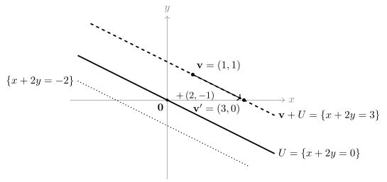
In , with
, the coset through is the line : a point
satisfies , and every solution of is of this
form with .
In general , so the cosets of are exactly the lines
parallel to .
The picture shows three cosets of : itself (solid), the
line through (dashed), and another parallel line
(dotted). The points and lie on the same dashed line, because
; so they are two representatives of
one coset. That observation is the
whole theory of cosets.
Lemma
4.4.3 (When two cosets are equal)
Let be a
subspace of . For
, write
if .
- (a) is an equivalence
relation on , and
the equivalence class of is the coset .
- (b) if and
only if .
- (c) Two cosets of
are either equal
or disjoint, and every vector of lies in exactly one
coset.
Proof.
(a) We check Definition 0.5.2. (E1)
.
(E2) If , then by Theorem 1.1.7 and
closure under scalar multiplication. (E3) If and , then by closure under addition. For the class,
means
for
some , that
is, ; so the class of Definition 0.5.3 is
.
(b) By (a) and Lemma 0.5.1 (a), if and
only if ,
that is, .
(c) This is Lemma 0.5.1 (b),
together with (take ).
More examples.
- Vertical lines. In , let , the
-axis. The coset
is
the vertical line through , and exactly when and . A coset is
determined by the shadow of any of its points on the
-plane.
- Polynomials with a prescribed
value. In , let , a subspace (the kernel of
evaluation at ).
Then
exactly when , that is, . So is the set of all polynomials with the same
constant term as .
- Degenerate cases. If , each coset
is
a single vector. If , there is only one coset, , because
always.
Non-example by minimal change. Try
to use the line , which is not a subspace, in place of
. The rule “ if ” is not
even reflexive: . What fails is the hypothesis that
is a subspace,
which (E1), (E2) and (E3) each used.
Warning. A coset has many
names, and it is usually not a subspace. In the
example above, and are the same set, although
.
Never conclude from ; conclude only . And is a subspace only
when it contains , that is, when and so . The dashed
line above is not a subspace.
The
quotient space
Now we want to treat each coset as a single point.
The motivation is a kind of deliberate forgetting.
Suppose we only care about vectors of “up to” adding
something from ,
for instance because we only ever measure the quantity
. Then and carry the same
information, and the space of all the information we
keep is the set of lines parallel to . We would like this set
to be a vector space, so that we can add and scale
lines.
The recipe is the one used for in Chapter 0 (Example (Addition modulo is well defined)):
define the operations through representatives, then
check that the choice of representatives does not
matter.
The quotient space is with everything in
declared to be
zero.
Definition
4.4.3 (Quotient space)
Let be a
subspace of a vector space over . The quotient
space
(read “ modulo
”) is the set of
all cosets of ,
with the operations The quotient map is ,
.
In words: an element of is a whole coset, a
subset of . By Lemma 4.4.3 (a),
is the quotient
set of by the
relation (Definition 0.5.5), and
is its quotient
map. To add two cosets, pick a representative of each,
add them in , and
take the coset of the result. To scale a coset, scale a
representative. The operations are written with
representatives, so before anything else we must check
that they are well defined.
The danger is real. By Lemma 4.4.3,
and
are one
element of .
If the sum depended on which of the two names we
used, the “definition” would assign two values to one
pair of cosets, and it would not define a function at
all (Definition 0.4.1). The
theorem below rules this out, and then shows that the
operations make
a vector space.
Theorem
4.4.4 (The Quotient Space Is a Vector
Space)
Let be a
subspace of a vector space over .
- (a) The addition and
scalar multiplication in Definition 4.4.3
are well defined: the right-hand sides depend only on
the cosets
and , not on
the representatives and .
- (b) With these
operations is a
vector space over . Its zero vector is
, and the
additive inverse of is .
- (c) The quotient map
is linear and surjective, and .
Idea. Chapter 0’s Theorem 0.5.3 turns a
function on that
is constant on classes into a function on . It is stated for
functions of one variable, so we use it one variable at
a time. ① For scalar multiplication by a fixed : if , then
. ② For addition, first freeze
the second summand and vary the first;
then show that the resulting function on cosets does not
change when is
replaced by an equivalent . Each check is
one line and uses exactly one closure property of . Once the operations
exist, every axiom for cosets is the same axiom in , passed through .
Proof. Throughout, means
,
and by Lemma 4.4.3 (b),
exactly when .
- (a) Scalar
multiplication. Fix , and let , . If
,
then by (VS5) and closure of under scalar
multiplication, so . By Theorem 0.5.3 (a),
there is exactly one function with for every . We define .
Addition, first variable. Fix , and let ,
. If , then , so
. By Theorem 0.5.3 (a),
there is exactly one function with for every .
Addition, second variable. Let be the set of all
functions , and let , .
Suppose . For every , , so Since every element of has the form , the functions
and are
equal, that is, . By Theorem 0.5.3 (a)
again, there is exactly one function
with . We define for . Then which is the formula of Definition 4.4.3,
and its value depends only on the two cosets.
- (b) Every element of
is for some
, and by (a) we
have and . Let
, , be in , and . Each axiom
follows by moving outside, using the
axiom in , and
moving back:
- (VS1) .
- (VS2) .
- (VS3) , so is a
zero vector.
- (VS4) , so is
an additive inverse of .
- (VS5) .
- (VS6) .
- (VS7) .
- (VS8) .
Hence is a
vector space over .
- (c) The identities
and from
(b) say that is
linear. It is surjective by the definition of . Finally, means
,
which by Lemma 4.4.3 (b)
means . So .
Part (c) has a pleasant reading: every
subspace is a kernel. Given , the
quotient map is a linear map whose kernel is exactly
.
Examples.
- Parallel lines. In with ,
write for
the line . Since , the definition gives and : to add two parallel lines, add their
“heights” and
. The zero vector
is .
- Constant terms. In with ,
the coset is
determined by ,
and is determined by . All that
survives of a polynomial is its constant term.
- Degenerate cases. has the cosets
, added
exactly as in :
nothing is forgotten. has the single
element , so it is
the zero space: everything is forgotten.
Non-example by minimal change.
Replace the line
by the union of the two axes, . It still contains and is still closed
under scalar multiplication, but it is not closed under
addition. Then “” is not transitive: and , but . Concretely, the “cosets” and both
contain , yet they are different sets, since
but would
need . The sets do not split into disjoint
pieces, so there is no set “” of the kind the
definition needs. The clause that fails is “ is a subspace”,
specifically closure under addition.
Why this definition. Each part of
the hypothesis that is a subspace has a
job: makes
reflexive;
closure under scalar multiplication makes symmetric and
scaling of cosets well defined; closure under addition
makes
transitive and addition of cosets well defined. The
non-example shows what goes wrong when one of them is
missing. The notation and the phrase
“modulo ” come
from ,
where integers are identified when their difference lies
in .
Warning. is not a subspace of
. Its
elements are subsets of , not vectors of , and its addition is a
new operation. For example, is not
the -plane: its
elements are vertical lines. The -plane is a
complement of the -axis, one of many
(Chapter 1), whereas involves no choice at
all. The two are isomorphic, as we show below, but they
are different objects.
In finite dimension the size of a quotient is exactly
what one would guess from the picture: we lose dimensions.
Theorem
4.4.5 (Dimension of a Quotient)
Let be
finite-dimensional and a subspace of . Then is finite-dimensional
and More precisely, if is a basis of such that is a
basis of , then
is a basis of .
Proof. By Theorem 4.4.4
(c), is linear, surjective and has kernel . By the Rank–Nullity
Theorem (Theorem 2.3.1), is
finite-dimensional and , which is the
formula.
For the basis, let and write . Since is linear and is the zero
vector, Theorem 2.1.4 gives
. So the list spans . Its length is , so it is a basis by Theorem 1.6.4
(b).
Such a basis always exists: take a basis of and extend it (Theorem 1.6.5). So
to find a basis of a quotient, extend a basis of
to one of and keep the cosets of
the new vectors.
Example
(A basis of a quotient of )
Let . Find a basis of , and write in it.
Solution. Extend by and . The list
is independent: in ,
the third entry gives , and then . It has length , so it is a basis of
(Theorem 1.6.4). By
Theorem 4.4.5,
is a basis of , which has
dimension .
To write , solve : the third entry
gives , then
and . Hence and indeed . The
coordinates
are
evaluated at : they are exactly the quantities that do
not change when a multiple of is added.
The warning above said that a quotient is not a
complement. The next result says how they are related:
any complement is a concrete model of the quotient.
Proposition
4.4.6 (A complement is a model of the
quotient)
Let be a
subspace of , and
let be a subspace
with . Then the restriction of the quotient map,
, , is an
isomorphism.
Proof. The restriction of the
linear map to
is linear.
Injective: if with , then by Lemma 4.4.3 (b),
so (Theorem 1.7.4); by
Theorem 2.2.3 the
restriction is injective. Surjective: given
, write with , ; then , so
. A
linear bijection is an isomorphism (Definition 2.5.2).
So every complement of is isomorphic to , which gives a second
proof that all complements have the same dimension. The
quotient is the choice-free object that all the
complements imitate.
Quick check. In with , is
? Is ? What is ?
Solution. By Lemma 4.4.3 (b):
, so the first two cosets are equal. , so the second pair are different cosets. By
Theorem 4.4.5,
.
The First
Isomorphism Theorem
A linear map forgets exactly the information in its
kernel: if and only if ,
that is, . In the language of this section, takes the same value at
two vectors exactly when they lie in the same coset of
. So is really a function of
the coset, and on cosets it forgets nothing.
Theorem
4.4.7 (First Isomorphism Theorem)
Let be a linear map, and let . Then the rule
defines a linear map, which is injective with
,
and satisfies . Hence
Proof. Well defined. is a subspace by Theorem 2.2.1, so
is a vector
space. If , then by Lemma 4.4.3 (b),
so . Hence is constant on each
coset of , and by
Theorem 0.5.3 (a)
there is exactly one function
with , that is, .
Linear. For and , by Definition 4.4.3
and the linearity of , and similarly .
Injective. If , then
, so and , the zero of
. By Theorem 2.2.3, is injective.
Image. The values of are the vectors
, , so .
Regarded as a map , is a linear bijection, hence an isomorphism
(Definition 2.5.2).
So every linear map factors as “collapse the kernel,
then embed”: , with surjective and injective. When
is
finite-dimensional, taking dimensions with Theorem 4.4.5
gives , which is Rank–Nullity again. The
theorem is stronger than the count, because it names the
isomorphism, and it holds in infinite dimension too.
The practical use runs the other way: to identify a
quotient , find
a surjective linear map out of whose kernel is exactly
.
Example
(Identifying quotients)
Use the First Isomorphism Theorem to show:
- (a) ,
where ;
- (b) , where .
Solution.
(a) Let ,
, which is linear because each entry is a
linear expression. It is surjective, since . Its
kernel is . By Theorem 4.4.7,
is an isomorphism . This
explains the coordinates found in Example (A basis of a quotient of ).
The check that it is well defined is visible: adding
to does not change
or .
(b) Let , . It is
linear by Theorem 0.8.5,
surjective because the constant polynomial maps to , and its kernel is
by definition. By
Theorem 4.4.7,
is an isomorphism .
In particular by Theorem 2.5.4, so
by Theorem 4.4.5.
The Second
and Third Isomorphism Theorems
Two more identifications come from the same method:
write down a surjective map, compute its kernel, and
apply the First Isomorphism Theorem. The first compares
a sum of subspaces with an intersection.
Theorem
4.4.8 (Second Isomorphism Theorem)
Let and be subspaces of a
vector space .
Then is a
subspace of ,
is a subspace of
, and is a well-defined isomorphism. Hence .
Idea. Picture two planes and in meeting in a line.
Modulo , a vector
of is
represented by its -part alone, since the
-part is
forgotten. The only vectors of that become zero are
those already in .
So the map “” from
is onto, with kernel .
Proof. is a subspace
(Theorem 1.2.2)
contained in , and
is a subspace
contained in
(Theorem 1.7.1), so
both quotients exist. Let be the quotient map, and let ,
, be
its restriction to ; is linear because is (Theorem 4.4.4).
is
surjective. An element of is with , . Since , Lemma 4.4.3 (b)
gives .
. For ,
means (Lemma 4.4.3 (b)),
that is, .
By Theorem 4.4.7
applied to , the
rule is a well-defined injective linear
map with image , hence an isomorphism. (Directly: if , then , so , and
the value does not depend on the representative.)
If and are finite-dimensional,
then so is
(it is spanned by the union of bases, Proposition 1.7.2),
and Theorem 4.4.5
turns the theorem into . That is the dimension formula
for sums (Theorem 1.7.3), now
as a consequence of an isomorphism rather than of a
basis computation. An exercise below asks for the
details.
The third theorem says that quotients can be taken in
stages.
Theorem
4.4.9 (Third Isomorphism Theorem)
Let be subspaces. Then is a subspace of , and is a well-defined isomorphism. Hence .
Proof. Let ,
.
Well defined. If ,
then , so by Lemma 4.4.3 (b).
By Theorem 0.5.3 (a),
applied to , , the rule defines a function on .
Linear and surjective. and similarly for scalars, by Definition 4.4.3
in both quotients. Every equals .
Kernel. means . If , then . Conversely, if with
, then
, so . Hence . In particular is a subspace of
, by Theorem 2.2.1.
By Theorem 4.4.7
applied to , , via .
The notation
is used with two meanings, and they agree: the quotient
space of by , and the set of cosets
with , sitting inside
. The coset
is the same
subset of in both
readings, and the operations agree because both are
computed with representatives. For example, with , the -axis and the -plane, through the
-coordinate, and
the theorem says that first forgetting and then forgetting
leaves the same
thing as forgetting both at once.
The
universal property of the quotient
The proofs of the three theorems repeated one move: a
linear map that vanishes on passes to . We record that move
once, in its general form. It is the standard way to
define linear maps out of a
quotient.
Theorem
4.4.10 (Universal Property of the
Quotient)
Let be a
subspace of ,
the quotient map, and a linear
map.
- (a) If , then
there is exactly one linear map
with , namely . Its image is , and it is
injective if and only if .
- (b) Conversely, if
some function satisfies ,
then .
Proof.
(a) If , then . By Theorem 0.5.3 (a)
there is exactly one function with , and
it is linear by the computation in the proof of Theorem 4.4.7,
which used only this formula. Any linear with
satisfies this formula, so it is this one. The image is
.
The kernel of is ; it is , the zero
subspace, exactly when every lies in
, that is, when
,
which together with means . Apply Theorem 2.2.3.
(b) Let . Then , so
by Theorem 2.1.1. Hence
.
In words: linear maps out of are the same as
linear maps out of that kill . The First
Isomorphism Theorem is the case . For example,
the map , , kills the -axis , so it induces , . Since is the -plane, strictly larger
than , this is not injective:
it also kills the coset .
Quotients will return in Chapter 9, where an operator
with induces
an operator on ,
and this is the engine of induction arguments on the
dimension.
Exercises
A. Check your
understanding
Exercise
(A1)
- (a) Define the
quotient space
and its two operations.
- (b) State the
condition, in terms of , for .
- (c) True or false:
is a subspace
of . Justify your
answer.
- (d) State the First
Isomorphism Theorem.
- (e) If is a -dimensional subspace of
, what is
? What
is ?
- (f) What must be
checked before the formula can be used as a definition, and which
property of makes
the check work?
Solution.
(a) For a
subspace of , , with and (Definition 4.4.3).
(b) if and
only if (Lemma 4.4.3).
(c) False. The
elements of are
cosets, which are subsets of , not vectors of .
(d) If is
linear, then is a well-defined isomorphism (Theorem 4.4.7).
(e) by Theorem 4.4.5,
and by Theorem 4.4.1.
(f) That the
right-hand side does not depend on the representatives:
if and , then . This works
because
and is closed
under addition.
B. Practice
Exercise
(B1: A basis of a quotient of )
Let .
- (a) Find and a basis
of .
- (b) Write in your
basis.
- (c) Decide whether
.
Solution.
(a) The two
spanning vectors are independent (look at the first two
entries), so and by Theorem 4.4.5.
Extend by . If , then from the last two entries and from the first
two. So the four vectors are independent, hence a basis
of (Theorem 1.6.4), and
by Theorem 4.4.5
is a basis of .
(b) Solve : ,
, , . Since the -part becomes zero in
the quotient, . Check: .
(c) The
difference is . A vector of has equal first and
third entries, but . So the difference is not in , and the cosets are
different by Lemma 4.4.3.
Exercise
(B2: A map that factors through a quotient)
Let , , and .
- (a) Show that , so
that induces a
linear map with .
- (b) Prove that is an
isomorphism.
- (c) Compute , and find
the coset .
Solution.
(a) is linear, since
evaluation and differentiation are. For , and ,
so , and
hence
for all . So , and
Theorem 4.4.10
(a) gives the linear map .
(b) and , so
is surjective and
. By Theorem 2.3.1, , so by Theorem 1.6.8. By Theorem 4.4.10
(a), is
injective with image . Hence is a linear bijection, an
isomorphism.
(c) . Since , , the set of all
.
Exercise
(B3: Matrices modulo scalars)
Let and
.
- (a) Show that is a subspace and find
.
- (b) For , find a basis of
.
- (c) Show that if and
only if is
a scalar matrix, and decide whether .
Solution.
(a) is a
subspace by Theorem 1.3.1, of
dimension since
. By Theorem 4.4.5,
.
(b) Extend by . If , then
and
then . So the
four matrices are independent, hence a basis of (Theorem 1.6.4), and
is a basis of by Theorem 4.4.5.
(c) This is Lemma 4.4.3 (b)
for the subspace .
Here the difference is , so the two
cosets are equal.
C. Going deeper
Exercise
(C1: The dimension formula from isomorphisms)
Let and be finite-dimensional
subspaces of a vector space .
- (a) Using Theorem 4.4.8 and
Theorem 4.4.5,
prove that .
- (b) Give a second
proof: apply Rank–Nullity to the addition map , , after showing that is
an isomorphism from onto .
Solution.
(a) is
finite-dimensional, being spanned by a basis of followed by a basis of
(Proposition 1.7.2),
and is finite-dimensional (Theorem 1.6.7). By
Theorem 4.4.8,
, and isomorphic finite-dimensional spaces
have equal dimension (Theorem 2.5.4).
Applying Theorem 4.4.5 to
both sides, which rearranges to the formula.
(b) The map is linear with image
by Theorem 4.4.2
(a). Let , ; it is well defined because and , and linear
because the operations are entrywise. It is injective,
since forces . Its image lies in , since .
Conversely, if , then ; so , hence and . Thus is an isomorphism onto
, and . By Theorem 4.4.1 and
Theorem 2.3.1,
Exercise
(C2: The operator induced on a quotient)
Let be
finite-dimensional, , and a subspace with for every .
- (a) Prove that is a well-defined linear operator on .
- (b) Let be a
basis of ,
extended to a basis of . Show that where is the matrix of the restriction in
, is the matrix of in , and
is the
zero matrix.
- (c) Check (b) when
is
differentiation on , with
and .
Hint: for (a), apply Theorem 4.4.10 to
.
Solution.
(a) The map , , is linear as a composition of linear maps
(Theorem 2.4.2). For
, , so ,
the zero of ;
thus . By Theorem 4.4.10
(a) there is exactly one linear map
with .
(b) For , , so it is a
combination of only, and its -coordinates are in the last places. These first
columns,
restricted to their first entries, are the
columns of the matrix of (which maps to by hypothesis and is
linear). For the remaining columns, write . Passing to , where is zero,
gives . So the matrix is the matrix
of in the basis of Theorem 4.4.5,
and the bottom-right block of is
.
(c) , , , so .
Differentiation maps into itself. The block is the matrix of on in , the lower-left
block is , and the block is the matrix : indeed , the zero coset, since .
Exercise
(C3: Counting cosets over a finite field)
Let be
a finite field with elements, a vector space over
of dimension
, and a subspace of dimension
.
- (a) Show that .
- (b) Show that every
coset has
exactly elements, and deduce by counting.
- (c) Check that (b)
agrees with Theorem 4.4.5.
Solution.
(a) Choose a
basis . By Theorem 1.5.1, is a bijection , and has elements.
(b) The map , , is
surjective by Definition 4.4.2
and injective because implies . So by (a) applied to . By Lemma 4.4.3 (c),
the cosets partition into
disjoint sets of size , so , and .
(c) By Theorem 4.4.5,
is a vector
space over of
dimension , so
by (a) it has elements, in agreement with (b). For
example,
modulo a line has cosets.