18.6 Linear Programming Duality

Chapter 3 ended its traffic example (Example (Traffic in a town center)) by admitting what linear algebra alone cannot do: “Non-negativity and street capacities turn the problem into one about inequalities, which is the subject of linear programming.” This section takes up that subject. A linear program asks for the largest value of a linear function on a region cut out by finitely many linear inequalities. The theory is almost entirely one idea. Every such maximum comes with a companion minimum, the dual program, and the two optimal values are equal. The proof of that equality is Farkas’s lemma of §05, applied to one combined system.

The equality has a practical meaning that goes beyond the theorem. A feasible point proves a lower bound on the maximum, a dual feasible point proves an upper bound, and when the two bounds meet, the answer has been certified: anyone can check it by multiplying out, with no need to trust how it was found.

Throughout, the field is $\mathbb{R}$ , vectors are columns, and $\mathbf{x} \ge \mathbf{0}$ , $\mathbf{u} \le \mathbf{v}$ are the entrywise relations of §05.

18.6.1. Linear programs

Here is a small instance of the kind of question we want to answer. A workshop makes two products. Each unit of the first uses $2$ hours of machine time and $1$ hour of labor, each unit of the second uses $1$ hour of machine time and $3$ hours of labor, and at most $3$ units of the first can be sold. Machine time is limited to $7$ hours, labor to $9$ , and the profits are $4$ and $3$ per unit. With $x_1, x_2$ units made, the question is: $\begin{aligned} \text{maximize}\quad & 4x_1 + 3x_2 \\ \text{subject to}\quad & 2x_1 + x_2 \le 7, \quad x_1 + 3x_2 \le 9, \quad x_1 \le 3, \\ & x_1 \ge 0, \quad x_2 \ge 0 . \end{aligned}$ The objective and every constraint are linear, and there are finitely many constraints. In matrix form it reads “maximize $\mathbf{c}^{\top}\mathbf{x}$ subject to $\mathbf{A}\mathbf{x} \le \mathbf{b}$ , $\mathbf{x} \ge \mathbf{0}$ ”. That shape deserves a name.

A linear program is the search for the best value of a linear function over a region defined by finitely many linear inequalities.

Definition 18.6.1 (Linear Program)

Let $\mathbf{A} \in M_{m \times n}(\mathbb{R})$ , $\mathbf{b} \in \mathbb{R}^m$ and $\mathbf{c} \in \mathbb{R}^n$ . The linear program with these data, in inequality form, is the problem $\text{(P)}\qquad \text{maximize } \mathbf{c}^{\top}\mathbf{x} \quad \text{subject to} \quad \mathbf{A}\mathbf{x} \le \mathbf{b},\ \ \mathbf{x} \ge \mathbf{0} .$ A vector $\mathbf{x} \in \mathbb{R}^n$ with $\mathbf{A}\mathbf{x} \le \mathbf{b}$ and $\mathbf{x} \ge \mathbf{0}$ is a feasible point, and the set of all of them is the feasible region. The program is feasible if it has a feasible point and infeasible otherwise. It is unbounded if it is feasible and $\mathbf{c}^{\top}\mathbf{x}$ takes arbitrarily large values on the feasible region. A feasible $\mathbf{x}^{\star}$ is an optimal solution if $\mathbf{c}^{\top}\mathbf{x}^{\star} \ge \mathbf{c}^{\top}\mathbf{x}$ for every feasible $\mathbf{x}$ , and then $\mathbf{c}^{\top}\mathbf{x}^{\star}$ is the optimal value.

Clause by clause. The function $\mathbf{x} \mapsto \mathbf{c}^{\top}\mathbf{x}$ is the objective. The $m$ rows of $\mathbf{A}\mathbf{x} \le \mathbf{b}$ are the constraints, and $\mathbf{x} \ge \mathbf{0}$ adds $n$ more. An optimal solution is a feasible point at which the objective is as large as anywhere on the feasible region, and it need not be unique. The optimal value is unique when it exists. A program can fail to have an optimal solution in two ways: it can have no feasible point, or its objective can be unbounded above. Whether those are the only two ways is the question the section’s second theorem settles.

Examples. The workshop problem is (P) with $\mathbf{A} = \begin{pmatrix} 2 & 1 \\ 1 & 3 \\ 1 & 0 \end{pmatrix}, \qquad \mathbf{b} = \begin{pmatrix} 7 \\ 9 \\ 3 \end{pmatrix}, \qquad \mathbf{c} = \begin{pmatrix} 4 \\ 3 \end{pmatrix} .$

One variable. With $n = m = 1$ , “maximize $x$ subject to $x \le 2$ , $x \ge 0$ ” has the optimal solution $x = 2$ . “Maximize $x$ subject to $-x \le -1$ , $x \ge 0$ ” asks for the largest $x \ge 1$ , and it is unbounded. “Maximize $x$ subject to $x \le -1$ , $x \ge 0$ ” is infeasible.
Degenerate case. If $\mathbf{c} = \mathbf{0}$ , every feasible point is optimal, with value $0$ . The program then asks only whether the system $\mathbf{A}\mathbf{x} \le \mathbf{b}$ , $\mathbf{x} \ge \mathbf{0}$ has a solution. So the feasibility question of Corollary 18.5.7 is itself a linear program, the one with no objective.

Non-example by minimal change. Make one inequality strict: “maximize $x$ subject to $x < 2$ , $x \ge 0$ ”. Everything is still linear, but the supremum $2$ is not attained, and no feasible point is optimal. The definition allows only non-strict inequalities. They define closed regions, and closedness will again be what the proofs need.

Why this form. Every problem with a linear objective and finitely many linear constraints can be brought to the shape (P). To minimize $\mathbf{c}^{\top}\mathbf{x}$ , maximize $(-\mathbf{c})^{\top}\mathbf{x}$ . A constraint $\mathbf{a}^{\top}\mathbf{x} \ge \beta$ is $(-\mathbf{a})^{\top}\mathbf{x} \le -\beta$ . An equation $\mathbf{a}^{\top}\mathbf{x} = \beta$ is the pair $\mathbf{a}^{\top}\mathbf{x} \le \beta$ , $-\mathbf{a}^{\top}\mathbf{x} \le -\beta$ . A variable $x_j$ without a sign constraint can be written $x_j = u_j - v_j$ with $u_j, v_j \ge 0$ . Exercise (C2: Free variables) carries out the last conversion. The form (P), with its sign constraints on $\mathbf{x}$ , is chosen because its dual, below, has the same shape, which makes the theory symmetric.

Example (The workshop problem, drawn)

Find the optimal solution of the workshop problem, and explain why it is optimal.

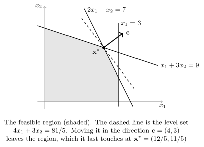
Solution. The feasible region is the pentagon with corners $(0, 0)$ , $(3, 0)$ , $(3, 1)$ , $\bigl(\tfrac{12}{5}, \tfrac{11}{5}\bigr)$ and $(0, 3)$ . For example, $(3, 1)$ is where $x_1 = 3$ meets $2x_1 + x_2 = 7$ , and $\bigl(\tfrac{12}{5}, \tfrac{11}{5}\bigr)$ solves $2x_1 + x_2 = 7$ , $x_1 + 3x_2 = 9$ : subtracting twice the second equation from the first gives $-5x_2 = -11$ .

$Diagram. Labels: x_1, x_2, x_1 + 3x_2 = 9, mathbf c, 2x_1 + x_2 = 7, x_1 = 3, mathbf x^star, The feasible region (shaded). The dashed line is the level set\\ 4x_1 + 3x_2 = 81/5. Moving it in the direction mathbf c = (4, 3)\\ leaves the region, which it last touches at mathbf x^star = (12/5, 11/5)$

The level sets $4x_1 + 3x_2 = \text{const}$ are parallel lines, and the value grows in the direction $\mathbf{c} = (4, 3)$ . Sliding the line in that direction, the last point of the region it meets appears to be $\mathbf{x}^{\star} = \bigl(\tfrac{12}{5}, \tfrac{11}{5}\bigr)$ , with value $4\cdot\tfrac{12}{5} + 3\cdot\tfrac{11}{5} = \tfrac{48 + 33}{5} = \tfrac{81}{5} .$ Comparing the corners supports this: they give $0$ , $12$ , $15$ , $\tfrac{81}{5} = 16.2$ and $9$ .

A picture is not a proof, and neither is a list of five corners, since we have not proved that an optimum sits at a corner. Here is a proof. Multiply the first constraint by $\tfrac95$ and the second by $\tfrac25$ , both non-negative, and add: $\tfrac95(2x_1 + x_2) + \tfrac25(x_1 + 3x_2) \le \tfrac95\cdot 7 + \tfrac25\cdot 9 = \tfrac{81}{5} .$ The left side is $\bigl(\tfrac{18}{5} + \tfrac25\bigr)x_1 + \bigl(\tfrac95 + \tfrac65\bigr)x_2 = 4x_1 + 3x_2$ . So every feasible point has $4x_1 + 3x_2 \le \tfrac{81}{5}$ , and $\mathbf{x}^{\star}$ , which is feasible ( $\tfrac{12}{5} \le 3$ as well), reaches this bound. It is optimal, and the optimal value is $\tfrac{81}{5}$ .

The multipliers $\tfrac95$ and $\tfrac25$ are the heart of the matter. They were chosen so that the combined constraint had exactly the objective as its left side. The best upper bound obtainable this way is itself the answer to a linear program.

18.6.2. The dual program

Multiply the $i$ -th constraint of (P) by a number $y_i \ge 0$ and add. For every feasible $\mathbf{x}$ this gives $\mathbf{y}^{\top}\mathbf{A}\mathbf{x} \le \mathbf{y}^{\top}\mathbf{b}$ . If the combination dominates the objective coefficient by coefficient, $\mathbf{A}^{\top}\mathbf{y} \ge \mathbf{c}$ , then, since $\mathbf{x} \ge \mathbf{0}$ , $\mathbf{c}^{\top}\mathbf{x} \le (\mathbf{A}^{\top}\mathbf{y})^{\top}\mathbf{x} = \mathbf{y}^{\top}\mathbf{A}\mathbf{x} \le \mathbf{y}^{\top}\mathbf{b} .$ Each such $\mathbf{y}$ proves an upper bound $\mathbf{b}^{\top}\mathbf{y}$ on the objective, and the natural question is how small that bound can be made.

The dual program searches for the best upper bound that non-negative combinations of the constraints can prove.

Definition 18.6.2 (Dual Program)

The dual of the linear program (P) of Definition 18.6.1 is the problem $\text{(D)}\qquad \text{minimize } \mathbf{b}^{\top}\mathbf{y} \quad \text{subject to} \quad \mathbf{A}^{\top}\mathbf{y} \ge \mathbf{c},\ \ \mathbf{y} \ge \mathbf{0} ,$ with $\mathbf{y} \in \mathbb{R}^m$ . The words feasible, infeasible and optimal are used as for (P). (D) is unbounded if it is feasible and $\mathbf{b}^{\top}\mathbf{y}$ takes arbitrarily negative values on its feasible region. In this context (P) is called the primal program.

The dual has one variable for each constraint of the primal and one constraint for each variable of the primal. The matrix is transposed, the roles of $\mathbf{b}$ and $\mathbf{c}$ are exchanged, and maximization becomes minimization. The dual of (D), written back in inequality form, is (P) again. Exercise (C1: The dual of the dual) checks this, and it explains why a statement about (P) always has a mirror statement about (D).

For the workshop problem the dual is $\begin{aligned} \text{minimize}\quad & 7y_1 + 9y_2 + 3y_3 \\ \text{subject to}\quad & 2y_1 + y_2 + y_3 \ge 4, \quad y_1 + 3y_2 \ge 3, \\ & y_1, y_2, y_3 \ge 0 , \end{aligned}$ and the multipliers of Example (The workshop problem, drawn) form the dual feasible point $\mathbf{y}^{\star} = \bigl(\tfrac95, \tfrac25, 0\bigr)$ , with $\mathbf{b}^{\top}\mathbf{y}^{\star} = \tfrac{81}{5}$ . The dual has an economic reading too. $y_i$ is a price for one unit of the $i$ -th resource, and the constraints say that at these prices the resources used by one unit of each product are worth at least the profit it brings.

18.6.3. Weak duality

The computation that motivated (D) is the first theorem, and it is one line long.

Theorem 18.6.1 (Weak Duality)

If $\mathbf{x}$ is feasible for (P) and $\mathbf{y}$ is feasible for (D), then $\mathbf{c}^{\top}\mathbf{x} \le \mathbf{b}^{\top}\mathbf{y} .$

Proof. Since $\mathbf{A}^{\top}\mathbf{y} - \mathbf{c} \ge \mathbf{0}$ and $\mathbf{x} \ge \mathbf{0}$ , the number $(\mathbf{A}^{\top}\mathbf{y} - \mathbf{c})^{\top}\mathbf{x}$ is a sum of products of non-negative numbers, so $\mathbf{c}^{\top}\mathbf{x} \le (\mathbf{A}^{\top}\mathbf{y})^{\top}\mathbf{x} = \mathbf{y}^{\top}(\mathbf{A}\mathbf{x})$ . Since $\mathbf{b} - \mathbf{A}\mathbf{x} \ge \mathbf{0}$ and $\mathbf{y} \ge \mathbf{0}$ , in the same way $\mathbf{y}^{\top}(\mathbf{A}\mathbf{x}) \le \mathbf{y}^{\top}\mathbf{b} = \mathbf{b}^{\top}\mathbf{y}$ . Chaining the two inequalities proves the theorem.

Corollary 18.6.2 (Certificates from Weak Duality)

(a) If $\mathbf{x}$ is feasible for (P), $\mathbf{y}$ is feasible for (D), and $\mathbf{c}^{\top}\mathbf{x} = \mathbf{b}^{\top}\mathbf{y}$ , then $\mathbf{x}$ is optimal for (P) and $\mathbf{y}$ is optimal for (D).
(b) If (P) is unbounded, then (D) is infeasible. If (D) is unbounded, then (P) is infeasible.

Idea. Weak duality makes every dual value an upper bound for every primal value. A primal value that meets one of these bounds cannot be beaten, and neither can the bound; an unbounded program leaves no room for any bound at all.

Proof.

(a) For every feasible $\mathbf{x}'$ , Theorem 18.6.1 gives $\mathbf{c}^{\top}\mathbf{x}' \le \mathbf{b}^{\top}\mathbf{y} = \mathbf{c}^{\top}\mathbf{x}$ , so $\mathbf{x}$ is optimal. For every dual feasible $\mathbf{y}'$ , it gives $\mathbf{b}^{\top}\mathbf{y}' \ge \mathbf{c}^{\top}\mathbf{x} = \mathbf{b}^{\top}\mathbf{y}$ , so $\mathbf{y}$ is optimal.
(b) If (D) had a feasible point $\mathbf{y}$ , Theorem 18.6.1 would bound $\mathbf{c}^{\top}\mathbf{x}$ above by $\mathbf{b}^{\top}\mathbf{y}$ for every feasible $\mathbf{x}$ , so (P) would not be unbounded. The second statement is the same argument with the roles exchanged.

Part (a) is exactly what Example (The workshop problem, drawn) did: $\mathbf{c}^{\top}\mathbf{x}^{\star} = \tfrac{81}{5} = \mathbf{b}^{\top}\mathbf{y}^{\star}$ , so both points are optimal. It gives a certificate of optimality that can be checked by arithmetic alone. The question is whether such a certificate always exists. Weak duality allows the best lower bound to stay strictly below the best upper bound.

Quick check. Without solving anything, give an upper bound for $4x_1 + 3x_2$ on the workshop’s feasible region using only the second constraint $x_1 + 3x_2 \le 9$ and $x \ge \mathbf{0}$ . Which dual feasible point is that?

Solution. We need $y_2 \ge 0$ with $y_2 \ge 4$ and $3y_2 \ge 3$ , so $y_2 = 4$ . Then $4x_1 + 3x_2 \le 4x_1 + 12x_2 = 4(x_1 + 3x_2) \le 36$ , using $x_2 \ge 0$ . This is the dual feasible point $\mathbf{y} = (0, 4, 0)$ , with $\mathbf{b}^{\top}\mathbf{y} = 36$ . It is a valid bound, but a poor one compared with the optimal $\tfrac{81}{5}$ .

18.6.4. Strong duality

The main theorem says that the gap allowed by weak duality never occurs, and it gives the complete list of what can happen.

Theorem 18.6.3 (Strong Duality for Linear Programs)

Let $\mathbf{A} \in M_{m \times n}(\mathbb{R})$ , $\mathbf{b} \in \mathbb{R}^m$ and $\mathbf{c} \in \mathbb{R}^n$ , and let (P) and (D) be as in Definition 18.6.1 and Definition 18.6.2.

(a) If (P) and (D) are both feasible, then both have optimal solutions, and their optimal values are equal: there are feasible $\mathbf{x}^{\star}$ and $\mathbf{y}^{\star}$ with $\mathbf{c}^{\top}\mathbf{x}^{\star} = \mathbf{b}^{\top}\mathbf{y}^{\star}$ .
(b) If (P) is feasible and (D) is infeasible, then (P) is unbounded.
(c) If (D) is feasible and (P) is infeasible, then (D) is unbounded.

Idea. Parts (b) and (c) are each one application of Corollary 18.5.7. The infeasibility of one program yields a vector that the other program can move along forever, with its objective improving without bound.

For (a) we want a single pair $(\mathbf{x}, \mathbf{y})$ that is feasible for both programs and has $\mathbf{c}^{\top}\mathbf{x} \ge \mathbf{b}^{\top}\mathbf{y}$ . Weak duality then forces equality, and Corollary 18.6.2 forces optimality. The pair is a solution of one big system of inequalities in $(\mathbf{x}, \mathbf{y})$ , so we ask Farkas whether it has one. If it had none, Farkas would hand us a certificate $(\mathbf{u}, \mathbf{v}, t)$ . The number $t$ is the multiplier on the row $\mathbf{b}^{\top}\mathbf{y} \le \mathbf{c}^{\top}\mathbf{x}$ . If $t > 0$ , rescaling the certificate by $1/t$ produces a primal and a dual feasible point that violate weak duality. If $t = 0$ , the certificate is a pair of directions along which one of the two programs is unbounded, which contradicts weak duality against a feasible point of the other.

Proof. (b) Let $\mathbf{x}_0$ be feasible for (P). That (D) is infeasible says that the system $(-\mathbf{A}^{\top})\mathbf{y} \le -\mathbf{c}$ , $\mathbf{y} \ge \mathbf{0}$ has no solution. By Corollary 18.5.7, applied with $\mathbf{M} = -\mathbf{A}^{\top}$ and $\mathbf{d} = -\mathbf{c}$ , there is $\mathbf{w} \in \mathbb{R}^n$ with $\mathbf{w} \ge \mathbf{0}$ , $(-\mathbf{A}^{\top})^{\top}\mathbf{w} = -\mathbf{A}\mathbf{w} \ge \mathbf{0}$ and $-\mathbf{c}^{\top}\mathbf{w} < 0$ . That is, $\mathbf{A}\mathbf{w} \le \mathbf{0}$ and $\mathbf{c}^{\top}\mathbf{w} > 0$ . For every $s \ge 0$ the point $\mathbf{x}_0 + s\mathbf{w}$ is feasible, since $\mathbf{A}(\mathbf{x}_0 + s\mathbf{w}) = \mathbf{A}\mathbf{x}_0 + s\mathbf{A}\mathbf{w} \le \mathbf{b}$ and $\mathbf{x}_0 + s\mathbf{w} \ge \mathbf{0}$ . Its objective value is $\mathbf{c}^{\top}\mathbf{x}_0 + s\,\mathbf{c}^{\top}\mathbf{w}$ , which is larger than any given number once $s$ is large enough, because $\mathbf{c}^{\top}\mathbf{w} > 0$ . So (P) is unbounded.

(c) Let $\mathbf{y}_0$ be feasible for (D). That (P) is infeasible says that $\mathbf{A}\mathbf{x} \le \mathbf{b}$ , $\mathbf{x} \ge \mathbf{0}$ has no solution. By Corollary 18.5.7 with $\mathbf{M} = \mathbf{A}$ and $\mathbf{d} = \mathbf{b}$ , there is $\mathbf{w} \in \mathbb{R}^m$ with $\mathbf{w} \ge \mathbf{0}$ , $\mathbf{A}^{\top}\mathbf{w} \ge \mathbf{0}$ and $\mathbf{b}^{\top}\mathbf{w} < 0$ . For $s \ge 0$ the point $\mathbf{y}_0 + s\mathbf{w}$ is feasible for (D), since $\mathbf{A}^{\top}(\mathbf{y}_0 + s\mathbf{w}) \ge \mathbf{A}^{\top}\mathbf{y}_0 \ge \mathbf{c}$ and $\mathbf{y}_0 + s\mathbf{w} \ge \mathbf{0}$ . Its value $\mathbf{b}^{\top}\mathbf{y}_0 + s\,\mathbf{b}^{\top}\mathbf{w}$ is below any given number for large $s$ . So (D) is unbounded.

(a) Let $\mathbf{x}_0$ be feasible for (P) and $\mathbf{y}_0$ feasible for (D). Consider the $(m + n + 1) \times (n + m)$ matrix and the vector $\mathbf{M} = \begin{pmatrix} \mathbf{A} & \mathbf{0} \\ \mathbf{0} & -\mathbf{A}^{\top} \\ -\mathbf{c}^{\top} & \mathbf{b}^{\top} \end{pmatrix}, \qquad \mathbf{d} = \begin{pmatrix} \mathbf{b} \\ -\mathbf{c} \\ 0 \end{pmatrix} .$ For $\mathbf{z} = (\mathbf{x}, \mathbf{y})$ with $\mathbf{x} \in \mathbb{R}^n$ and $\mathbf{y} \in \mathbb{R}^m$ , the system $\mathbf{M}\mathbf{z} \le \mathbf{d}$ , $\mathbf{z} \ge \mathbf{0}$ says exactly that

\mathbf{A}\mathbf{x} \le \mathbf{b}, \quad \mathbf{A}^{\top}\mathbf{y} \ge \mathbf{c}, \quad \mathbf{b}^{\top}\mathbf{y} \le \mathbf{c}^{\top}\mathbf{x}, \quad \mathbf{x} \ge \mathbf{0}, \quad \mathbf{y} \ge \mathbf{0} .

(18.6.1)

Suppose Eq. 18.6.1 has a solution $(\mathbf{x}^{\star}, \mathbf{y}^{\star})$ . Then $\mathbf{x}^{\star}$ is feasible for (P) and $\mathbf{y}^{\star}$ is feasible for (D), so Theorem 18.6.1 gives $\mathbf{c}^{\top}\mathbf{x}^{\star} \le \mathbf{b}^{\top}\mathbf{y}^{\star}$ . Together with $\mathbf{b}^{\top}\mathbf{y}^{\star} \le \mathbf{c}^{\top}\mathbf{x}^{\star}$ , this gives equality, and by Corollary 18.6.2 (a) both points are optimal. That is (a).

It remains to show that Eq. 18.6.1 has a solution. Suppose not. By Corollary 18.5.7 there is $\mathbf{w} \ge \mathbf{0}$ with $\mathbf{M}^{\top}\mathbf{w} \ge \mathbf{0}$ and $\mathbf{d}^{\top}\mathbf{w} < 0$ . Write $\mathbf{w} = (\mathbf{u}, \mathbf{v}, t)$ with $\mathbf{u} \in \mathbb{R}^m$ , $\mathbf{v} \in \mathbb{R}^n$ and $t \in \mathbb{R}$ , all $\ge 0$ . Since $\mathbf{M}^{\top} = \begin{pmatrix} \mathbf{A}^{\top} & \mathbf{0} & -\mathbf{c} \\ \mathbf{0} & -\mathbf{A} & \mathbf{b} \end{pmatrix} ,$ the conditions read

\mathbf{A}^{\top}\mathbf{u} \ge t\mathbf{c}, \qquad \mathbf{A}\mathbf{v} \le t\mathbf{b}, \qquad \mathbf{b}^{\top}\mathbf{u} < \mathbf{c}^{\top}\mathbf{v} .

(18.6.2)

Case 1: $t > 0$ . Dividing Eq. 18.6.2 by $t$ shows that $\mathbf{v}/t \ge \mathbf{0}$ is feasible for (P), that $\mathbf{u}/t \ge \mathbf{0}$ is feasible for (D), and that $\mathbf{b}^{\top}(\mathbf{u}/t) < \mathbf{c}^{\top}(\mathbf{v}/t)$ . This contradicts Theorem 18.6.1.

Case 2: $t = 0$ . Now $\mathbf{A}^{\top}\mathbf{u} \ge \mathbf{0}$ , $\mathbf{A}\mathbf{v} \le \mathbf{0}$ and $\mathbf{b}^{\top}\mathbf{u} < \mathbf{c}^{\top}\mathbf{v}$ , with $\mathbf{u}, \mathbf{v} \ge \mathbf{0}$ . The strict inequality forces $\mathbf{c}^{\top}\mathbf{v} > 0$ or $\mathbf{b}^{\top}\mathbf{u} < 0$ , since otherwise $\mathbf{b}^{\top}\mathbf{u} \ge 0 \ge \mathbf{c}^{\top}\mathbf{v}$ . If $\mathbf{c}^{\top}\mathbf{v} > 0$ , then, exactly as in the proof of (b), the points $\mathbf{x}_0 + s\mathbf{v}$ with $s \ge 0$ are feasible for (P) with objective values tending to $+\infty$ . That contradicts the bound $\mathbf{c}^{\top}\mathbf{x} \le \mathbf{b}^{\top}\mathbf{y}_0$ that Theorem 18.6.1 gives for every feasible $\mathbf{x}$ . If $\mathbf{b}^{\top}\mathbf{u} < 0$ , then, as in the proof of (c), the points $\mathbf{y}_0 + s\mathbf{u}$ are feasible for (D) with values tending to $-\infty$ , which contradicts $\mathbf{b}^{\top}\mathbf{y} \ge \mathbf{c}^{\top}\mathbf{x}_0$ .

Both cases are impossible, so Eq. 18.6.1 has a solution, and (a) is proved. This proves the theorem.

Together with Corollary 18.6.2 (b), the theorem sorts every pair (P), (D) into exactly one of four cases:

(P)	(D)	what happens
feasible	feasible	both optimal, equal values (a)
feasible	infeasible	(P) unbounded (b)
infeasible	feasible	(D) unbounded (c)
infeasible	infeasible	nothing more to say

All four occur. The workshop problem is the first. The one-variable program “maximize $x$ subject to $-x \le -1$ , $x \ge 0$ ” is the second: its dual, “minimize $-y$ subject to $-y \ge 1$ , $y \ge 0$ ”, is infeasible. “Maximize $0 \cdot x$ subject to $x \le -1$ , $x \ge 0$ ” is the third: its dual, “minimize $-y$ subject to $y \ge 0$ ”, is unbounded. For the fourth, take $\mathbf{A} = \begin{pmatrix} 1 & -1 \\ -1 & 1 \end{pmatrix}, \qquad \mathbf{b} = \begin{pmatrix} -1 \\ -1 \end{pmatrix}, \qquad \mathbf{c} = \begin{pmatrix} 1 \\ 1 \end{pmatrix} .$ Adding the two primal constraints gives $0 \le -2$ , and adding the two dual constraints gives $0 \ge 2$ , so neither program is feasible.

The table has a consequence that is easy to state and not at all obvious.

Corollary 18.6.4 (Bounded Linear Programs Attain Their Optimum)

If (P) is feasible and its objective is bounded above on the feasible region, that is, $\mathbf{c}^{\top}\mathbf{x} \le N$ for some $N$ and every feasible $\mathbf{x}$ , then (P) has an optimal solution. The same holds for (D) with “bounded below”.

Proof. Since (P) is feasible and not unbounded, part (b) of Theorem 18.6.3 shows that (D) is not infeasible. So both programs are feasible, and part (a) gives an optimal solution of (P). The statement for (D) follows in the same way from part (c).

Why is this not obvious? The feasible region is closed, but it may be unbounded, so the extreme value theorem (A4) of Chapter 16’s introduction does not apply to it. And a linear function that is bounded above on a closed convex set need not attain its supremum. On the region $R = \{ (x_1, x_2) : x_1 > 0,\ x_1x_2 \ge 1 \}$ , bounded by a branch of a hyperbola, the linear function $-x_2$ is negative everywhere, and it takes values arbitrarily close to $0$ at the points $(k, 1/k)$ , so its supremum is $0$ . That supremum is never reached. The region $R$ is the set $A$ of Example (A hyperbola and its asymptote), since $x_1 > 0$ and $x_1x_2 \ge 1$ force $x_2 > 0$ , and that example shows it is closed and convex. But it is not cut out by finitely many linear inequalities. That finiteness is what made the cones in the proof finitely generated, and hence closed, by Theorem 18.5.4. The corollary is where finite generation pays off.

Warning. Strong duality is a theorem about linear programs, not about optimization in general. For programs whose objective or constraints are convex but not linear, one can still write down a dual problem, and weak duality still holds, but the two optimal values may differ: a duality gap. Extra hypotheses are needed to close it, of which the best known is a strictly feasible point (Slater’s condition). That theory belongs to convex optimization and is not developed in this book. For linear programs no hypothesis beyond feasibility is needed, as Theorem 18.6.3 shows.

18.6.5. Complementary slackness

Strong duality says that at the optimum the two chains of inequalities in the proof of Theorem 18.6.1 are equalities. Reading that off term by term gives a test that locates the dual solution once the primal one is known.

Theorem 18.6.5 (Complementary Slackness)

Let $\mathbf{x}$ be feasible for (P) and $\mathbf{y}$ feasible for (D). Then $\mathbf{x}$ and $\mathbf{y}$ are both optimal if and only if

(i) for every $i$ , $y_i > 0$ implies $(\mathbf{A}\mathbf{x})_i = b_i$ ; and
(ii) for every $j$ , $x_j > 0$ implies $(\mathbf{A}^{\top}\mathbf{y})_j = c_j$ .

Idea. The gap $\mathbf{b}^{\top}\mathbf{y} - \mathbf{c}^{\top}\mathbf{x}$ is a sum of products of non-negative numbers, one product for each constraint of either program. Optimality means the gap is zero, which means every product is zero.

Proof. Expanding and using $\mathbf{y}^{\top}\mathbf{A}\mathbf{x} = \mathbf{x}^{\top}\mathbf{A}^{\top}\mathbf{y}$ ,

\mathbf{b}^{\top}\mathbf{y} - \mathbf{c}^{\top}\mathbf{x} = \mathbf{y}^{\top}(\mathbf{b} - \mathbf{A}\mathbf{x}) + \mathbf{x}^{\top}(\mathbf{A}^{\top}\mathbf{y} - \mathbf{c}) .

(18.6.3)

The first term on the right is $\sum_i y_i(\mathbf{b} - \mathbf{A}\mathbf{x})_i$ , a sum of products of non-negative numbers, and so is the second. Condition (i) says that every product in the first sum is zero, and (ii) says the same for the second. So (i) and (ii) together hold exactly when the right side of Eq. 18.6.3 is $0$ , because a sum of non-negative numbers is zero only when every term is.

$(\Leftarrow)$ If (i) and (ii) hold, then $\mathbf{c}^{\top}\mathbf{x} = \mathbf{b}^{\top}\mathbf{y}$ , and both points are optimal by Corollary 18.6.2 (a).

$(\Rightarrow)$ If both are optimal, then both programs are feasible, and by Theorem 18.6.3 (a) their optimal values are equal. So $\mathbf{c}^{\top}\mathbf{x} = \mathbf{b}^{\top}\mathbf{y}$ , the right side of Eq. 18.6.3 is $0$ , and (i) and (ii) hold.

In words: a constraint with a positive price must be tight, and a product that is actually made must exactly pay for its resources. For the workshop problem, $\mathbf{x}^{\star} = \bigl(\tfrac{12}{5}, \tfrac{11}{5}\bigr)$ has both entries positive, so (ii) requires both dual constraints to be tight: $2y_1 + y_2 + y_3 = 4, \qquad y_1 + 3y_2 = 3 .$ The third primal constraint is slack at $\mathbf{x}^{\star}$ , since $\tfrac{12}{5} < 3$ , so (i) forces $y_3 = 0$ . The two equations then give $y_1 = \tfrac95$ and $y_2 = \tfrac25$ , both $\ge 0$ , which recovers the multipliers of Example (The workshop problem, drawn). So the multipliers were not a lucky guess: complementary slackness finds them from the primal solution.

18.6.6. Traffic, with inequalities

We return to Chapter 3’s town center, to answer the remark made there. Recall from Example (Traffic in a town center) the four intersections, the five one-way streets $1 \to 2$ , $2 \to 3$ , $3 \to 4$ , $4 \to 1$ , $1 \to 3$ with flows $f_1, \dots, f_5$ , and the incidence matrix $\mathbf{N}$ . Conservation of cars is $\mathbf{N}\mathbf{f} = \mathbf{s}$ with $\mathbf{s} = (40, 20, -35, -25)$ , and the flows that conserve cars are $\mathbf{f} = (40 - \beta + \alpha,\ 60 - \beta + \alpha,\ 25 + \alpha,\ \alpha,\ \beta), \qquad \alpha, \beta \in \mathbb{R} .$ Chapter 3 asked, with street $4 \to 1$ closed, for the largest possible flow on the diagonal $1 \to 3$ , and found $40$ by inspecting the one remaining parameter. That was already a linear program: maximize $f_5$ subject to $\mathbf{N}\mathbf{f} = \mathbf{s}$ , $\mathbf{f} \ge \mathbf{0}$ , $f_4 = 0$ . Its answer has a one-line certificate. The first row of $\mathbf{N}\mathbf{f} = \mathbf{s}$ , the balance at intersection 1, reads $f_1 - f_4 + f_5 = 40$ , so $f_5 = 40 - f_1 + f_4 = 40 - f_1 \le 40$ because $f_1 \ge 0$ .

Example (Capacities on every street)

Suppose street $4 \to 1$ is open again, but every street can carry at most $35$ cars per minute. What is the smallest flow the diagonal street $1 \to 3$ can carry, and how would you convince someone that it cannot be smaller?

Solution. The linear program is: minimize $f_5$ subject to $\mathbf{N}\mathbf{f} = \mathbf{s}$ and $\mathbf{0} \le \mathbf{f} \le 35\cdot\mathbf{1}$ . In the parameters, the capacity of street $2 \to 3$ reads $60 - \beta + \alpha \le 35$ , so $\beta \ge 25 + \alpha \ge 25$ , since $\alpha = f_4 \ge 0$ . The value $\beta = 25$ is achieved: with $\alpha = 0$ the flow is $\mathbf{f} = (15, 35, 25, 0, 25) ,$ every entry of which lies between $0$ and $35$ . So the minimum is $25$ .

The certificate, in the spirit of the dual, is a non-negative combination of the constraints. Add the balance equations at intersections 1 and 2, $f_1 - f_4 + f_5 = 40$ and $-f_1 + f_2 = 20$ : $f_2 - f_4 + f_5 = 60, \qquad\text{so}\qquad f_5 = 60 - f_2 + f_4 \ \ge\ 60 - 35 + 0 = 25 ,$ using the capacity $f_2 \le 35$ and the sign constraint $f_4 \ge 0$ . In words: at least sixty cars per minute arrive at the pair of intersections $\{1, 2\}$ (sixty from outside, plus whatever street $4 \to 1$ brings), and only two streets leave that pair, $2 \to 3$ and the diagonal. The first can take at most $35$ , so the diagonal must take at least $25$ . This is a cut argument, and it is exactly what the dual program of a flow problem computes. The balance equations carry multipliers of either sign, the “potentials” of the intersections, and here they are $1$ at intersections 1 and 2 and $0$ at the others.

This is the answer to Chapter 3’s remark. Linear algebra describes the conserving flows as a coset of the null space of $\mathbf{N}$ . Linear programming chooses among them, and duality explains each choice with a certificate that can be read as a statement about the network.

Remark. Computing optimal solutions of large linear programs is a subject in its own right. The best known method, the simplex method, moves from corner to corner of the feasible region, each time improving the objective. This book does not develop algorithms for linear programming. Section 9 returns to the corners themselves, as the vertices of a polyhedron.

18.6.7. Exercises

A. Check your understanding

Exercise (A1)

(a) Write down the dual of: maximize $2x_1 + x_2$ subject to $x_1 + x_2 \le 3$ , $x_1 - x_2 \le 1$ , $\mathbf{x} \ge \mathbf{0}$ .
(b) State weak duality and strong duality.
(c) Determine whether the following is correct, and justify your answer: if (P) is infeasible, then (D) is unbounded.
(d) Determine whether the following is correct, and justify your answer: if (P) is feasible and $\mathbf{c}^{\top}\mathbf{x} \le 100$ for every feasible $\mathbf{x}$ , then (P) has an optimal solution.
(e) At an optimal pair $\mathbf{x}, \mathbf{y}$ , suppose $x_2 > 0$ . What does complementary slackness say about the second constraint of (D)?

Solution.

(a) Minimize $3y_1 + y_2$ subject to $y_1 + y_2 \ge 2$ , $y_1 - y_2 \ge 1$ , $\mathbf{y} \ge \mathbf{0}$ . The columns of $\mathbf{A}$ become the rows of $\mathbf{A}^{\top}$ , and $\mathbf{b} = (3, 1)$ and $\mathbf{c} = (2, 1)$ exchange roles.
(b) Weak duality (Theorem 18.6.1): if $\mathbf{x}$ is feasible for (P) and $\mathbf{y}$ for (D), then $\mathbf{c}^{\top}\mathbf{x} \le \mathbf{b}^{\top}\mathbf{y}$ . Strong duality (Theorem 18.6.3): if both are feasible, both have optimal solutions with equal values. If exactly one is feasible, that one is unbounded.
(c) Incorrect. Both programs can be infeasible, as for $\mathbf{A} = \begin{psmallmatrix} 1 & -1 \\ -1 & 1\end{psmallmatrix}$ , $\mathbf{b} = (-1, -1)$ , $\mathbf{c} = (1, 1)$ in this section. What is true, by Theorem 18.6.3 (c), is that if (P) is infeasible and (D) is feasible, then (D) is unbounded.
(d) Correct, by Corollary 18.6.4. The bound shows that (P) is not unbounded, so by Theorem 18.6.3 (b) the dual is feasible, and then (a) gives an optimal solution.
(e) By Theorem 18.6.5 (ii), the second dual constraint is tight: $(\mathbf{A}^{\top}\mathbf{y})_2 = c_2$ .

B. Practice

Exercise (B1: Solve and certify)

Consider: maximize $x_1 + 2x_2$ subject to $x_1 + x_2 \le 5, \qquad -x_1 + x_2 \le 1, \qquad 2x_1 - x_2 \le 4, \qquad \mathbf{x} \ge \mathbf{0} .$

(a) Sketch the feasible region and guess an optimal solution.
(b) Write down the dual, and use complementary slackness to find a candidate dual solution.
(c) Prove that both candidates are optimal, and state the optimal value.

Solution.

(a) The region is the pentagon with corners $(0, 0)$ , $(2, 0)$ , $(3, 2)$ , $(2, 3)$ and $(0, 1)$ , where the objective takes the values $0, 2, 7, 8, 2$ . The guess is $\mathbf{x}^{\star} = (2, 3)$ , where $x_1 + x_2 = 5$ meets $-x_1 + x_2 = 1$ .
(b) The dual is: minimize $5y_1 + y_2 + 4y_3$ subject to $y_1 - y_2 + 2y_3 \ge 1$ , $y_1 + y_2 - y_3 \ge 2$ , $\mathbf{y} \ge \mathbf{0}$ . At $\mathbf{x}^{\star}$ the third constraint is slack, since $2\cdot 2 - 3 = 1 < 4$ , so (i) of Theorem 18.6.5 requires $y_3 = 0$ . Both $x_j^{\star} > 0$ , so (ii) requires both dual constraints to be tight: $y_1 - y_2 = 1$ and $y_1 + y_2 = 2$ . Hence $\mathbf{y}^{\star} = \bigl(\tfrac32, \tfrac12, 0\bigr)$ .
(c) $\mathbf{x}^{\star}$ is feasible: $5 \le 5$ , $1 \le 1$ , $1 \le 4$ , and $\mathbf{x}^{\star} \ge \mathbf{0}$ . $\mathbf{y}^{\star}$ is feasible: $\mathbf{y}^{\star} \ge \mathbf{0}$ , $\tfrac32 - \tfrac12 = 1 \ge 1$ and $\tfrac32 + \tfrac12 = 2 \ge 2$ . The objective values are $\mathbf{c}^{\top}\mathbf{x}^{\star} = 2 + 6 = 8$ and $\mathbf{b}^{\top}\mathbf{y}^{\star} = \tfrac{15}{2} + \tfrac12 = 8$ . They are equal, so both points are optimal by Corollary 18.6.2 (a), and the optimal value is $8$ .

Exercise (B2: Which case?)

For each program, write down its dual, and determine which of the four cases of Theorem 18.6.3 occurs. Justify your answer, giving the optimal values where they exist.

(a) Maximize $x_1 + x_2$ subject to $x_1 - x_2 \le 1$ , $\mathbf{x} \ge \mathbf{0}$ .
(b) Maximize $-x_1$ subject to $x_1 \le 2$ , $-x_1 \le -1$ , $x_1 \ge 0$ .
(c) Maximize $x_1$ subject to $x_1 + x_2 \le -1$ , $\mathbf{x} \ge \mathbf{0}$ .

Solution.

(a) The dual is: minimize $y$ subject to $y \ge 1$ , $-y \ge 1$ , $y \ge 0$ . The last two constraints conflict, so the dual is infeasible. The primal is feasible, with $\mathbf{0}$ a feasible point, so by Theorem 18.6.3 (b) it is unbounded. Directly, $(0, s)$ is feasible for every $s \ge 0$ , with value $s$ .
(b) The dual is: minimize $2y_1 - y_2$ subject to $y_1 - y_2 \ge -1$ , $\mathbf{y} \ge \mathbf{0}$ . Both programs are feasible: $x_1 = 1$ and $\mathbf{y} = (0, 1)$ . Their values are $-1$ and $2\cdot 0 - 1 = -1$ , which are equal, so both are optimal by Corollary 18.6.2 (a), with optimal value $-1$ . This is the first case.
(c) The primal is infeasible, since $x_1 + x_2 \ge 0 > -1$ for $\mathbf{x} \ge \mathbf{0}$ . The dual is: minimize $-y$ subject to $y \ge 1$ , $y \ge 0$ , $y \ge 0$ . It is feasible, and $-y$ takes arbitrarily negative values, so it is unbounded, as Theorem 18.6.3 (c) predicts.

Exercise (B3: A network with one flow)

In the traffic network of this section, close street $4 \to 1$ and give every other street a capacity of $30$ cars per minute. Show that there is exactly one feasible flow. For its diagonal flow $f_5 = 30$ , give a certificate, in the style of Example (Capacities on every street), that $f_5 \ge 30$ for every feasible flow, and one that $f_5 \le 30$ .

Solution. With $f_4 = \alpha = 0$ the conserving flows are $\mathbf{f} = (40 - \beta, 60 - \beta, 25, 0, \beta)$ . The capacity of street $2 \to 3$ gives $60 - \beta \le 30$ , so $\beta \ge 30$ . The capacity of the diagonal gives $\beta \le 30$ . So $\beta = 30$ , and the only candidate is $\mathbf{f} = (10, 30, 25, 0, 30)$ , which satisfies $0 \le f_i \le 30$ for every street. It is the unique feasible flow.

Lower bound: adding the balance equations at intersections 1 and 2 gives $f_2 - f_4 + f_5 = 60$ , so $f_5 = 60 - f_2 + f_4 = 60 - f_2 \ge 30$ by the capacity $f_2 \le 30$ , using $f_4 = 0$ . Upper bound: $f_5 \le 30$ is itself a capacity constraint. Each certificate is a non-negative combination of constraints, with free multipliers on the balance equations, as in the example.

C. Going deeper

Exercise (C1: The dual of the dual)

(a) Rewrite (D) as a program in the inequality form of Definition 18.6.1, with data $(-\mathbf{A}^{\top}, -\mathbf{c}, -\mathbf{b})$ . Show that the dual of that program, rewritten as a maximization, is (P).
(b) Deduce part (c) of Theorem 18.6.3 from part (b).

Solution.

(a) Minimizing $\mathbf{b}^{\top}\mathbf{y}$ is maximizing $(-\mathbf{b})^{\top}\mathbf{y}$ , and $\mathbf{A}^{\top}\mathbf{y} \ge \mathbf{c}$ is $(-\mathbf{A}^{\top})\mathbf{y} \le -\mathbf{c}$ . So (D) is the inequality-form program (D $'$ ): maximize $(-\mathbf{b})^{\top}\mathbf{y}$ subject to $(-\mathbf{A}^{\top})\mathbf{y} \le -\mathbf{c}$ , $\mathbf{y} \ge \mathbf{0}$ , whose data are $\mathbf{A}' = -\mathbf{A}^{\top}$ , $\mathbf{b}' = -\mathbf{c}$ , $\mathbf{c}' = -\mathbf{b}$ . By Definition 18.6.2 its dual is: minimize $\mathbf{b}'^{\top}\mathbf{x} = (-\mathbf{c})^{\top}\mathbf{x}$ subject to $\mathbf{A}'^{\top}\mathbf{x} = -\mathbf{A}\mathbf{x} \ge \mathbf{c}' = -\mathbf{b}$ , $\mathbf{x} \ge \mathbf{0}$ . That is: maximize $\mathbf{c}^{\top}\mathbf{x}$ subject to $\mathbf{A}\mathbf{x} \le \mathbf{b}$ , $\mathbf{x} \ge \mathbf{0}$ , which is (P). Its optimal value is the negative of the minimum above.
(b) Suppose (D) is feasible and (P) is infeasible. Then (D $'$ ) is feasible, with the same feasible points, and its dual, which by (a) has the same feasible points as (P), is infeasible. By Theorem 18.6.3 (b) applied to (D $'$ ), the objective $(-\mathbf{b})^{\top}\mathbf{y}$ takes arbitrarily large values on the feasible region. So $\mathbf{b}^{\top}\mathbf{y}$ takes arbitrarily negative values, and (D) is unbounded.

Exercise (C2: Free variables)

Let $\mathbf{A} \in M_{m \times n}(\mathbb{R})$ , $\mathbf{b} \in \mathbb{R}^m$ , $\mathbf{c} \in \mathbb{R}^n$ , and consider the program with no sign constraint on $\mathbf{x}$ : $\text{(P}_{\text{free}}\text{)}\qquad \text{maximize } \mathbf{c}^{\top}\mathbf{x} \ \text{ subject to } \ \mathbf{A}\mathbf{x} \le \mathbf{b} .$

(a) Prove weak duality between (P $_{\text{free}}$ ) and (D $_{\text{eq}}$ ): minimize $\mathbf{b}^{\top}\mathbf{y}$ subject to $\mathbf{A}^{\top}\mathbf{y} = \mathbf{c}$ , $\mathbf{y} \ge \mathbf{0}$ .
(b) Writing $\mathbf{x} = \mathbf{u} - \mathbf{v}$ with $\mathbf{u}, \mathbf{v} \ge \mathbf{0}$ , show that (P $_{\text{free}}$ ) has the same values as an inequality-form program whose dual is (D $_{\text{eq}}$ ). Deduce that if both are feasible, both have optimal solutions with equal values.

Solution.

(a) If $\mathbf{A}\mathbf{x} \le \mathbf{b}$ and $\mathbf{A}^{\top}\mathbf{y} = \mathbf{c}$ with $\mathbf{y} \ge \mathbf{0}$ , then $\mathbf{c}^{\top}\mathbf{x} = (\mathbf{A}^{\top}\mathbf{y})^{\top}\mathbf{x} = \mathbf{y}^{\top}\mathbf{A}\mathbf{x} \le \mathbf{y}^{\top}\mathbf{b}$ , the last step because $\mathbf{y} \ge \mathbf{0}$ and $\mathbf{b} - \mathbf{A}\mathbf{x} \ge \mathbf{0}$ . No sign condition on $\mathbf{x}$ is needed, because the first step is an equality.
(b) Every $\mathbf{x} \in \mathbb{R}^n$ can be written as $\mathbf{u} - \mathbf{v}$ with $\mathbf{u}, \mathbf{v} \ge \mathbf{0}$ : take $u_j = \max(x_j, 0)$ and $v_j = \max(-x_j, 0)$ . So (P $_{\text{free}}$ ) has the same feasible objective values as the inequality-form program $\text{maximize } \begin{pmatrix} \mathbf{c} \\ -\mathbf{c} \end{pmatrix}^{\top}\begin{pmatrix} \mathbf{u} \\ \mathbf{v} \end{pmatrix} \ \text{ subject to } \ \begin{pmatrix} \mathbf{A} & -\mathbf{A} \end{pmatrix}\begin{pmatrix} \mathbf{u} \\ \mathbf{v} \end{pmatrix} \le \mathbf{b}, \quad \begin{pmatrix} \mathbf{u} \\ \mathbf{v} \end{pmatrix} \ge \mathbf{0} ,$ with an optimal $(\mathbf{u}, \mathbf{v})$ giving an optimal $\mathbf{x} = \mathbf{u} - \mathbf{v}$ , and conversely. By Definition 18.6.2 its dual is: minimize $\mathbf{b}^{\top}\mathbf{y}$ subject to $\begin{pmatrix} \mathbf{A} & -\mathbf{A}\end{pmatrix}^{\top}\mathbf{y} \ge (\mathbf{c}, -\mathbf{c})$ , $\mathbf{y} \ge \mathbf{0}$ . The constraint reads $\mathbf{A}^{\top}\mathbf{y} \ge \mathbf{c}$ and $-\mathbf{A}^{\top}\mathbf{y} \ge -\mathbf{c}$ , that is, $\mathbf{A}^{\top}\mathbf{y} = \mathbf{c}$ . So the dual is (D $_{\text{eq}}$ ). If both programs are feasible, Theorem 18.6.3 (a) gives optimal $(\mathbf{u}^{\star}, \mathbf{v}^{\star})$ and $\mathbf{y}^{\star}$ with equal values, and $\mathbf{x}^{\star} = \mathbf{u}^{\star} - \mathbf{v}^{\star}$ is optimal for (P $_{\text{free}}$ ).