5.4 The Dual Map and the Transpose

So far each space has had its own dual, but the duals of different spaces have not talked to each other. Linear algebra is about maps, so the question is: what does a linear map $T \colon V \to W$ do to functionals? This section shows that $T$ moves vectors forward but moves measurements backward, giving the dual map $T' \colon W^{*} \to V^{*}$ . In dual bases its matrix is the transpose of the matrix of $T$ , which finally explains what the transpose of Chapter 0 means. The kernel and image of $T'$ are annihilators of the image and kernel of $T$ , and counting dimensions gives a third proof that row rank equals column rank. At the end we return to the double dual and prove that the evaluation map is compatible with every linear map.

5.4.1. Pulling functionals back

After spaces come the maps between them. We have a linear map $T \colon V \to W$ and the two spaces of measurements $V^{*}$ and $W^{*}$ . We want to know how $T$ relates them.

Start with the standard example, a matrix map $T_{\mathbf{A}} \colon F^n \to F^m$ , $\mathbf{x} \mapsto \mathbf{A}\mathbf{x}$ , with $\mathbf{A} \in M_{m \times n}(F)$ . A functional on $F^m$ is $\psi(\mathbf{y}) = \mathbf{b}^{\top}\mathbf{y}$ for a unique $\mathbf{b} \in F^m$ (Theorem 5.1.1). Given $\psi$ , there is one obvious way to measure a vector $\mathbf{x} \in F^n$ : move it to $F^m$ with $T_{\mathbf{A}}$ , then measure. The result is $\psi(T_{\mathbf{A}}\mathbf{x}) = \mathbf{b}^{\top} \mathbf{A}\mathbf{x} = (\mathbf{A}^{\top}\mathbf{b})^{\top}\mathbf{x},$ using $(\mathbf{A}^{\top}\mathbf{b})^{\top} = \mathbf{b}^{\top} \mathbf{A}$ (Theorem 0.9.5). So “move, then measure” is again a functional, now on $F^n$ , and it is given by the vector $\mathbf{A}^{\top}\mathbf{b}$ . The transpose appears by itself. The recipe “compose with $T$ ” makes sense for any linear map, and it deserves a name.

The dual map pulls a measurement of $W$ back to a measurement of $V$ : first move the vector with $T$ , then measure it in $W$ .

Definition 5.4.1 (Dual Map)

Let $V$ and $W$ be vector spaces over $F$ , and let $T \in \mathcal{L}(V, W)$ . The dual map of $T$ is the map $T' \colon W^{*} \to V^{*}, \qquad T'(\psi) \mathrel{:=} \psi T = \psi \circ T .$ That is, $(T'\psi)(\mathbf{v}) = \psi(T\mathbf{v})$ for every $\psi \in W^{*}$ and every $\mathbf{v} \in V$ .

In words, clause by clause:

The input of $T'$ is a functional on the codomain $W$ , and the output is a functional on the domain $V$ . The arrow is reversed.
The formula $(T'\psi)(\mathbf{v}) = \psi(T\mathbf{v})$ has two steps: to measure $\mathbf{v}$ with $T'\psi$ , send $\mathbf{v}$ to $W$ with $T$ , then apply $\psi$ there.
No basis and no finite dimension are involved.

Well-definedness. Two things must be checked. First, $T'\psi$ must lie in $V^{*}$ : it is the composite of the linear maps $T \colon V \to W$ and $\psi \colon W \to F$ , so it is linear by Theorem 2.4.2 (a). Second, $T'$ should be linear, so that $T' \in \mathcal{L}(W^{*}, V^{*})$ . By the distributive laws in Theorem 2.4.2 (d), for $\psi_1, \psi_2 \in W^{*}$ and $c \in F$ , $\begin{aligned} T'(\psi_1 + \psi_2) &= (\psi_1 + \psi_2)T = \psi_1T + \psi_2T = T'\psi_1 + T'\psi_2, \\ T'(c\psi) &= (c\psi)T = c(\psi T) = cT'\psi . \end{aligned}$

Example (Dual Maps in Four Settings)

(a) For $\mathbf{A} \in M_{m \times n}(F)$ , describe $T_{\mathbf{A}}'$ in terms of the vectors $\mathbf{b}$ and $\mathbf{A}^{\top}\mathbf{b}$ that represent functionals.
(b) Let $D \colon \mathbb{R}[x]_{\le 3} \to \mathbb{R}[x]_{\le 2}$ , $D(p) = p'$ , and let $\varepsilon_2 \in (\mathbb{R}[x]_{\le 2})^{*}$ be $\varepsilon_2(q) = q(2)$ . Compute $D'(\varepsilon_2)$ .
(c) Let $S \colon F[x] \to F[x]$ , $S(p) = xp$ , and let $\varphi_k \in F[x]^{*}$ send a polynomial to its coefficient of $x^k$ . Compute $S'(\varphi_k)$ for every $k \in \mathbb{N}$ .
(d) Find $(\operatorname{id}_V)'$ , the dual map of the zero map $V \to W$ , and the dual map of the inclusion $\iota \colon U \to V$ , $\iota(\mathbf{u}) = \mathbf{u}$ , of a subspace $U \subseteq V$ .

Solution.

(a) If $\psi(\mathbf{y}) = \mathbf{b}^{\top}\mathbf{y}$ , the computation before the definition shows $(T_{\mathbf{A}}'\psi)(\mathbf{x}) = (\mathbf{A}^{\top}\mathbf{b})^{\top}\mathbf{x}$ . So, identifying a functional with its vector, $T_{\mathbf{A}}'$ is $\mathbf{b} \mapsto \mathbf{A}^{\top}\mathbf{b}$ . In row language: $T_{\mathbf{A}}'$ sends the row $\mathbf{b}^{\top}$ to the row $\mathbf{b}^{\top} \mathbf{A}$ .
(b) For $p \in \mathbb{R}[x]_{\le 3}$ , $(D'\varepsilon_2)(p) = \varepsilon_2(Dp) = p'(2)$ . So $D'$ turns “the value at $2$ ” into “the slope at $2$ ”.
(c) $(S'\varphi_k)(p) = \varphi_k(xp)$ . Multiplying by $x$ shifts every coefficient up one place, so the coefficient of $x^k$ in $xp$ is the coefficient of $x^{k-1}$ in $p$ when $k \ge 1$ , and $0$ when $k = 0$ . Hence $S'\varphi_k = \varphi_{k-1}$ for $k \ge 1$ , and $S'\varphi_0 = 0$ . Here $F[x]$ is infinite-dimensional, and the definition works all the same.
(d) $(\operatorname{id}_V)'\varphi = \varphi \circ \operatorname{id}_V = \varphi$ , so $(\operatorname{id}_V)' = \operatorname{id}_{V^{*}}$ . For the zero map $0 \colon V \to W$ , $(0'\psi)(\mathbf{v}) = \psi(\mathbf{0}) = 0$ (Theorem 2.1.1), so $0'$ is the zero map $W^{*} \to V^{*}$ . For the inclusion, $(\iota'\varphi)(\mathbf{u}) = \varphi(\mathbf{u})$ for $\mathbf{u} \in U$ , so $\iota'\varphi = \varphi|_U$ is the restriction of $\varphi$ to $U$ . The restriction map $V^{*} \to U^{*}$ is thus a dual map; we study it further in the next section.

Here is a non-example by minimal change. Try to push functionals forward instead: for $T \colon V \to W$ and $\varphi \in V^{*}$ , look for a $\psi \in W^{*}$ with $\psi T = \varphi$ , and call it “ $T_{*}\varphi$ ”. Take $T \colon \mathbb{R} \to \mathbb{R}^2$ , $T(t) = (t, 0)$ , and $\varphi(t) = t$ . Then $\psi(x, y) = x + cy$ satisfies $\psi(T(t)) = t$ for every $c \in \mathbb{R}$ , so there is no single answer. And for the zero map $\mathbb{R} \to \mathbb{R}^2$ , no $\psi$ at all satisfies $\psi \circ 0 = \varphi$ . What fails is well-definedness: a function must assign exactly one value. Composition with $T$ goes only one way, on the right, and that forces the direction $W^{*} \to V^{*}$ .

Why this definition. From $T \colon V \to W$ and $\psi \colon W \to F$ , the only composite we can form is $\psi T$ ; the non-example shows that the other direction is not a function. Linearity of $T'$ comes for free from the distributive laws. The name “dual map” says that $T'$ is the map $T$ induces between the duals. It is also called the transpose of $T$ , for a reason that the matrix theorem below makes exact. We write $T'$ rather than $T^{*}$ , because $T^{*}$ is reserved for the adjoint of Chapter 11, which is related to $T'$ but needs an inner product.

Warning. The dual map goes backwards. For $T \colon V \to W$ , the dual map is $T' \colon W^{*} \to V^{*}$ , not $V^{*} \to W^{*}$ . As a result, composition reverses order: if $T \colon U \to V$ and $S \colon V \to W$ , then $(ST)' = T'S'$ , just as $(\mathbf{A}\mathbf{B})^{\top} = \mathbf{B}^{\top} \mathbf{A}^{\top}$ . The other order $S'T'$ does not even make sense: $T'$ lands in $U^{*}$ , where $S'$ is not defined.

Quick check. Let $T \colon \mathbb{R}^3 \to \mathbb{R}^2$ , $T(x, y, z) = (x - z, 2y)$ , and $\psi(u, v) = u + v$ . Compute $T'\psi$ . If $T'$ is written as a matrix in some bases, what is its size?

Solution. $(T'\psi)(x, y, z) = \psi(x - z, 2y) = x + 2y - z$ . The map $T'$ goes from $(\mathbb{R}^2)^{*}$ , of dimension $2$ , to $(\mathbb{R}^3)^{*}$ , of dimension $3$ (Corollary 5.1.4), so its matrix is $3 \times 2$ , the size of the transpose of the $2 \times 3$ matrix of $T$ .

The first payoff is that duals behave well under the operations on maps, with one reversal.

Theorem 5.4.1 (Properties of the Dual Map)

Let $U, V, W$ be vector spaces over $F$ .

(a) For $S, T \in \mathcal{L}(V, W)$ and $a, b \in F$ , $(aS + bT)' = aS' + bT'$ .
(b) For $T \in \mathcal{L}(U, V)$ and $S \in \mathcal{L}(V, W)$ , $(ST)' = T'S'$ .
(c) $(\operatorname{id}_V)' = \operatorname{id}_{V^{*}}$ .
(d) If $T \in \mathcal{L}(V, W)$ is invertible, then $T'$ is invertible and $(T')^{-1} = (T^{-1})'$ .

Idea. Each identity is an equality of maps into a dual space, so we evaluate both sides at a functional, and then evaluate the resulting functionals at a vector. After that, each line is the definition of $T'$ read twice. Part (d) needs no computation: apply (b) and (c) to $T^{-1}T = \operatorname{id}_V$ and $TT^{-1} = \operatorname{id}_W$ .

Proof.

(a) Let $\psi \in W^{*}$ and $\mathbf{v} \in V$ . Using the linearity of $\psi$ and the pointwise operations (Definition 2.4.1), $\bigl((aS + bT)'\psi\bigr)(\mathbf{v}) = \psi(aS\mathbf{v} + bT\mathbf{v}) = a\psi(S\mathbf{v}) + b\psi(T\mathbf{v}) = \bigl(aS'\psi + bT'\psi\bigr)(\mathbf{v}).$ Hence $(aS + bT)'\psi = (aS' + bT')\psi$ for every $\psi$ , and $(aS + bT)' = aS' + bT'$ .
(b) Let $\psi \in W^{*}$ . By Definition 5.4.1 and associativity of composition (Theorem 2.4.2 (b)), $(ST)'\psi = \psi(ST) = (\psi S)T = T'(\psi S) = T'(S'\psi) = (T'S')\psi .$ Hence $(ST)' = T'S'$ .
(c) This is Example (Dual Maps in Four Settings) (d).
(d) Suppose $T$ is invertible with inverse $T^{-1} \in \mathcal{L}(W, V)$ . By (b) and (c), $T'(T^{-1})' = (T^{-1}T)' = (\operatorname{id}_V)' = \operatorname{id}_{V^{*}}, \qquad (T^{-1})'T' = (TT^{-1})' = (\operatorname{id}_W)' = \operatorname{id}_{W^{*}} .$ The map $(T^{-1})'$ is linear, so by Definition 2.5.1 $T'$ is invertible with inverse $(T^{-1})'$ . This proves the theorem.

Part (a) says that $T \mapsto T'$ is itself a linear map $\mathcal{L}(V, W) \to \mathcal{L}(W^{*}, V^{*})$ . Part (b) is the reversal of the warning. Parts (c) and (d) say that dualizing turns isomorphisms into isomorphisms, so isomorphic spaces have isomorphic duals.

5.4.2. The matrix of the dual map

Now we fix bases and compute. Let $\mathcal{B} = (\mathbf{v}_1, \dots, \mathbf{v}_n)$ be a basis of $V$ with dual basis $\mathcal{B}^{*} = (\varphi_1, \dots, \varphi_n)$ (Definition 5.1.3), and $\mathcal{C} = (\mathbf{w}_1, \dots, \mathbf{w}_m)$ a basis of $W$ with dual basis $\mathcal{C}^{*} = (\psi_1, \dots, \psi_m)$ . The map $T$ has the $m \times n$ matrix $[T]_{\mathcal{B}}^{\mathcal{C}}$ (Definition 4.1.1). The dual map $T' \colon W^{*} \to V^{*}$ has input basis $\mathcal{C}^{*}$ and output basis $\mathcal{B}^{*}$ , so its matrix is $[T']_{\mathcal{C}^{*}}^{\mathcal{B}^{*}}$ , of size $n \times m$ . The size already suggests the answer, and Example (Dual Maps in Four Settings) (a) suggests it for matrix maps.

Theorem 5.4.2 (The Matrix of the Dual Map Is the Transpose)

Let $V$ and $W$ be finite-dimensional vector spaces over $F$ , with ordered bases $\mathcal{B}$ of $V$ and $\mathcal{C}$ of $W$ , and let $\mathcal{B}^{*}$ and $\mathcal{C}^{*}$ be their dual bases. For every $T \in \mathcal{L}(V, W)$ , $[T']_{\mathcal{C}^{*}}^{\mathcal{B}^{*}} = \left([T]_{\mathcal{B}}^{\mathcal{C}}\right)^{\top} .$

Idea. Both matrices are tables of the same numbers $\psi_i(T\mathbf{v}_j)$ . In $[T]_{\mathcal{B}}^{\mathcal{C}}$ , the $(i, j)$ entry is the $\mathbf{w}_i$ -coordinate of $T\mathbf{v}_j$ , and a dual basis vector reads off a coordinate: that coordinate is $\psi_i(T\mathbf{v}_j)$ . In $[T']_{\mathcal{C}^{*}}^{\mathcal{B}^{*}}$ , column $i$ holds the $\mathcal{B}^{*}$ -coordinates of $T'\psi_i$ , and the $\varphi_j$ -coordinate of a functional is its value at $\mathbf{v}_j$ : that is $(T'\psi_i)(\mathbf{v}_j) = \psi_i(T\mathbf{v}_j)$ . The same number sits at $(i, j)$ in one matrix and at $(j, i)$ in the other.

Proof. Write $\mathcal{B} = (\mathbf{v}_1, \dots, \mathbf{v}_n)$ , $\mathcal{B}^{*} = (\varphi_1, \dots, \varphi_n)$ , $\mathcal{C} = (\mathbf{w}_1, \dots, \mathbf{w}_m)$ , $\mathcal{C}^{*} = (\psi_1, \dots, \psi_m)$ , and $\mathbf{A} = (a_{kj}) = [T]_{\mathcal{B}}^{\mathcal{C}}$ . By Definition 4.1.1, $a_{ij}$ is the $i$ -th entry of $[T\mathbf{v}_j]_{\mathcal{C}}$ , and by Theorem 5.1.3 (a) that entry is read off by $\psi_i$ : $\psi_i(T\mathbf{v}_j) = a_{ij} . \tag{$\ast$}$ Next, by Theorem 5.1.3 (c), every $\varphi \in V^{*}$ satisfies $\varphi = \sum_{j=1}^{n} \varphi(\mathbf{v}_j)\varphi_j$ . Since $\mathcal{B}^{*}$ is a basis, coordinates in it are unique (Theorem 1.5.1), so $[\varphi]_{\mathcal{B}^{*}} = (\varphi(\mathbf{v}_1), \dots, \varphi(\mathbf{v}_n))$ .

By Definition 4.1.1, column $i$ of $[T']_{\mathcal{C}^{*}}^{\mathcal{B}^{*}}$ is $[T'\psi_i]_{\mathcal{B}^{*}}$ . By the previous paragraph and $(\ast)$ , its $j$ -th entry is $(T'\psi_i)(\mathbf{v}_j) = \psi_i(T\mathbf{v}_j) = a_{ij} .$ So the $(j, i)$ entry of $[T']_{\mathcal{C}^{*}}^{\mathcal{B}^{*}}$ is $a_{ij}$ , which is the $(j, i)$ entry of $\mathbf{A}^{\top}$ (Definition 0.9.10). Both matrices are $n \times m$ , so $[T']_{\mathcal{C}^{*}}^{\mathcal{B}^{*}} = \mathbf{A}^{\top}$ . This proves the theorem.

This is the meaning of the transpose. In Chapter 0, Definition 0.9.10 was a rule for rearranging entries. Now we see it as the matrix shadow of pulling functionals back: transposing a matrix is dualizing the map, provided we use dual bases on both sides. Every property of the transpose becomes a property of dual maps, and conversely; for instance, Theorem 5.4.1 (b) and this theorem together give $(\mathbf{A}\mathbf{B})^{\top} = \mathbf{B}^{\top} \mathbf{A}^{\top}$ a second time (Exercise B3 below).

Example (A

2 \times 3

Example)

Let $T \colon \mathbb{R}[x]_{\le 2} \to \mathbb{R}^2$ , $T(p) = (p(1), p'(1))$ . Use the basis $\mathcal{B} = (1, x, x^2)$ , whose dual basis $\mathcal{B}^{*} = (\varphi_0, \varphi_1, \varphi_2)$ consists of $\varphi_0(p) = p(0)$ , $\varphi_1(p) = p'(0)$ , $\varphi_2(p) = p''(0)/2$ (Example (Dual Bases in $\mathbb{R}[x]_{\le 2}$ )), and the standard basis $\mathcal{C} = (\mathbf{e}_1, \mathbf{e}_2)$ of $\mathbb{R}^2$ , with dual basis $\mathcal{C}^{*} = (\eta_1, \eta_2)$ , $\eta_1(u, v) = u$ , $\eta_2(u, v) = v$ .

(a) Find $\mathbf{A} = [T]_{\mathcal{B}}^{\mathcal{C}}$ .
(b) Compute $T'\eta_1$ and $T'\eta_2$ directly as combinations of $\varphi_0, \varphi_1, \varphi_2$ , write down $[T']_{\mathcal{C}^{*}}^{\mathcal{B}^{*}}$ , and compare with $\mathbf{A}^{\top}$ .
(c) Use the matrix to compute $T'\psi$ for $\psi = -2\eta_1 + \eta_2$ , and check the answer directly.

Solution.

(a) $T(1) = (1, 0)$ , $T(x) = (1, 1)$ , $T(x^2) = (1, 2)$ . These are the columns: $\mathbf{A} = [T]_{\mathcal{B}}^{\mathcal{C}} = \begin{pmatrix} 1 & 1 & 1 \\ 0 & 1 & 2 \end{pmatrix}.$
(b) Let $p = a + bx + cx^2$ , so $\varphi_0(p) = a$ , $\varphi_1(p) = b$ , $\varphi_2(p) = c$ . Then $\begin{aligned} (T'\eta_1)(p) &= \eta_1(Tp) = p(1) = a + b + c, \\ (T'\eta_2)(p) &= \eta_2(Tp) = p'(1) = b + 2c . \end{aligned}$ So $T'\eta_1 = \varphi_0 + \varphi_1 + \varphi_2$ and $T'\eta_2 = \varphi_1 + 2\varphi_2$ . Their coordinate vectors in $\mathcal{B}^{*}$ are the columns of $[T']_{\mathcal{C}^{*}}^{\mathcal{B}^{*}} = \begin{pmatrix} 1 & 0 \\ 1 & 1 \\ 1 & 2 \end{pmatrix} = \mathbf{A}^{\top},$ as Theorem 5.4.2 predicts. Read in words, the first column is Taylor’s formula $p(1) = p(0) + p'(0) + \tfrac12 p''(0)$ for quadratics, and the second is $p'(1) = p'(0) + p''(0)$ .
(c) $[\psi]_{\mathcal{C}^{*}} = (-2, 1)$ . By Theorem 4.1.1, $[T'\psi]_{\mathcal{B}^{*}} = \mathbf{A}^{\top}\begin{pmatrix} -2 \\ 1 \end{pmatrix} = \begin{pmatrix} -2 \\ -1 \\ 0 \end{pmatrix},$ so $T'\psi = -2\varphi_0 - \varphi_1$ . Directly: $(T'\psi)(p) = -2p(1) + p'(1) = -2(a + b + c) + (b + 2c) = -2a - b$ , which is $(-2\varphi_0 - \varphi_1)(p)$ .

Warning. Dual bases on both sides. The transpose rule needs the dual bases $\mathcal{C}^{*}$ and $\mathcal{B}^{*}$ . With other bases of $W^{*}$ and $V^{*}$ the matrix of $T'$ is usually not $\mathbf{A}^{\top}$ . In Example (A $2 \times 3$ Example), keep $\mathcal{B}^{*}$ but use the basis $(\eta_1 + \eta_2, \eta_2)$ of $(\mathbb{R}^2)^{*}$ : then $T'(\eta_1 + \eta_2) = \varphi_0 + 2\varphi_1 + 3\varphi_2$ , so the first column is $(1, 2, 3)$ , not the first column $(1, 1, 1)$ of $\mathbf{A}^{\top}$ .

5.4.3. Kernel and image of the dual map

The kernel and image of $T'$ are subspaces of $W^{*}$ and $V^{*}$ . The natural candidates for them are annihilators of the subspaces that $T$ defines, and the dictionary swaps kernel and image.

Theorem 5.4.3 (Kernel and Image of the Dual Map)

Let $V$ and $W$ be vector spaces over $F$ , and let $T \in \mathcal{L}(V, W)$ .

(a) $\operatorname{ker} T' = (\operatorname{im} T)^{0}$ .
(b) If $V$ and $W$ are finite-dimensional, then $\operatorname{im} T' = (\operatorname{ker} T)^{0}$ .

Idea.

(a) is a chain of definitions: $\psi T = 0$ says that $\psi$ vanishes on every $T\mathbf{v}$ , that is, on $\operatorname{im} T$ . For (b), one inclusion is just as easy: $\psi T$ kills every vector that $T$ kills. The reverse inclusion asks us to extend a functional given on $V$ to one of the form $\psi T$ , which is a construction. Instead we count. Rank–Nullity for $T'$ , together with (a) and the dimension formula for annihilators, gives $\dim \operatorname{im} T' = \operatorname{rank} T$ ; the dimension formula in $V$ and Rank–Nullity for $T$ give $\dim (\operatorname{ker} T)^{0} = \operatorname{rank} T$ . Finite dimension is spent exactly on these counts.

Proof.

(a) Let $\psi \in W^{*}$ . Then $\psi \in \operatorname{ker} T'$ iff $\psi T = 0$ iff $\psi(T\mathbf{v}) = 0$ for every $\mathbf{v} \in V$ iff $\psi(\mathbf{w}) = 0$ for every $\mathbf{w} \in \operatorname{im} T$ (Definition 2.2.2) iff $\psi \in (\operatorname{im} T)^{0}$ (Definition 5.2.1).
(b) Let $n = \dim V$ and $m = \dim W$ , so $\dim V^{*} = n$ and $\dim W^{*} = m$ (Corollary 5.1.4).

Inclusion. Let $\varphi \in \operatorname{im} T'$ , say $\varphi = \psi T$ with $\psi \in W^{*}$ . For $\mathbf{u} \in \operatorname{ker} T$ , $\varphi(\mathbf{u}) = \psi(T\mathbf{u}) = \psi(\mathbf{0}) = 0$ . Hence $\varphi \in (\operatorname{ker} T)^{0}$ , and $\operatorname{im} T' \subseteq (\operatorname{ker} T)^{0}$ .

Dimensions. By the Rank–Nullity Theorem (Theorem 2.3.1) for $T' \colon W^{*} \to V^{*}$ , then (a), then Theorem 5.2.2 for the subspace $\operatorname{im} T$ of $W$ , $\begin{aligned} \dim \operatorname{im} T' &= m - \dim \operatorname{ker} T' = m - \dim (\operatorname{im} T)^{0} \\ &= m - (m - \dim \operatorname{im} T) = \operatorname{rank} T . \end{aligned}$ By Theorem 5.2.2 for the subspace $\operatorname{ker} T$ of $V$ , and Rank–Nullity for $T$ , $\dim (\operatorname{ker} T)^{0} = n - \dim \operatorname{ker} T = \operatorname{rank} T .$ So $\operatorname{im} T'$ is a subspace of the finite-dimensional space $(\operatorname{ker} T)^{0}$ with the same dimension, and Theorem 1.6.8 gives $\operatorname{im} T' = (\operatorname{ker} T)^{0}$ . This proves the theorem.

For a matrix map, this is a statement about rows. By Example (Dual Maps in Four Settings) (a), $T_{\mathbf{A}}'$ sends the row $\mathbf{b}^{\top}$ to $\mathbf{b}^{\top} \mathbf{A}$ , so $\operatorname{im} T_{\mathbf{A}}'$ is the set of combinations of the rows of $\mathbf{A}$ : it is the row space, read as functionals. Part (b) then says that the functionals vanishing on $\operatorname{nul}(\mathbf{A})$ are exactly the combinations of the rows of $\mathbf{A}$ . Part (a) says that the functionals vanishing on $\operatorname{col}(\mathbf{A})$ are the rows $\mathbf{b}^{\top}$ with $\mathbf{b}^{\top} \mathbf{A} = 0$ , that is, $\mathbf{A}^{\top}\mathbf{b} = \mathbf{0}$ .

Example (Kernel and Image of a Dual Map)

Let $T = T_{\mathbf{A}} \colon \mathbb{R}^3 \to \mathbb{R}^3$ with $\mathbf{A} = \begin{pmatrix} 1 & 0 & 2 \\ 0 & 1 & -1 \\ 1 & 1 & 1 \end{pmatrix}.$ Find bases of $\operatorname{ker} T'$ and $\operatorname{im} T'$ , written as explicit functionals, and check Theorem 5.4.3.

Solution. The matrix world. The third row of $\mathbf{A}$ is the sum of the first two, and subtracting them leaves the RREF $\begin{pmatrix} 1 & 0 & 2 \\ 0 & 1 & -1 \\ 0 & 0 & 0 \end{pmatrix}$ . So $\operatorname{rank} \mathbf{A} = 2$ , and $\mathbf{A}\mathbf{x} = \mathbf{0}$ gives $x = -2z$ , $y = z$ : $\operatorname{ker} T = \operatorname{span}\bigl((-2, 1, 1)\bigr)$ . The pivot columns give $\operatorname{im} T = \operatorname{span}\bigl((1, 0, 1), (0, 1, 1)\bigr)$ (Theorem 3.5.2).

Kernel of $T'$ . By Theorem 5.4.2 with standard bases and Example (Matrix Maps and the Identity) (a), a functional $\psi(u, v, w) = b_1u + b_2v + b_3w$ lies in $\operatorname{ker} T'$ iff $\mathbf{A}^{\top}\mathbf{b} = \mathbf{0}$ : $b_1 + b_3 = 0, \qquad b_2 + b_3 = 0, \qquad 2b_1 - b_2 + b_3 = 0 .$ The first two give $\mathbf{b} = t(1, 1, -1)$ , and these satisfy the third. So $\operatorname{ker} T' = \operatorname{span}(\psi_0)$ with $\psi_0(u, v, w) = u + v - w$ . Check: $\psi_0(1, 0, 1) = 0$ and $\psi_0(0, 1, 1) = 0$ , so $\psi_0$ vanishes on $\operatorname{im} T$ ; and $\dim (\operatorname{im} T)^{0} = 3 - 2 = 1$ (Theorem 5.2.2). So $\operatorname{ker} T' = (\operatorname{im} T)^{0}$ .

Image of $T'$ . By Example (Dual Maps in Four Settings) (a), $\operatorname{im} T'$ is spanned by the rows of $\mathbf{A}$ read as functionals, and the first two rows already span (the third is their sum): $\varphi_1(x, y, z) = x + 2z, \qquad \varphi_2(x, y, z) = y - z .$ They are independent (neither is a multiple of the other), so $(\varphi_1, \varphi_2)$ is a basis of $\operatorname{im} T'$ . Check: $\varphi_1(-2, 1, 1) = 0$ and $\varphi_2(-2, 1, 1) = 0$ , so both vanish on $\operatorname{ker} T$ , and $\dim (\operatorname{ker} T)^{0} = 3 - 1 = 2$ . So $\operatorname{im} T' = (\operatorname{ker} T)^{0}$ .

Counting dimensions in the proof of Theorem 5.4.3 already gave $\dim \operatorname{im} T' = \operatorname{rank} T$ . We record it, together with its most famous consequence.

Corollary 5.4.4 (Rank of the Dual Map)

(a) Let $V$ and $W$ be finite-dimensional vector spaces over $F$ , and $T \in \mathcal{L}(V, W)$ . Then $\operatorname{rank} T' = \operatorname{rank} T$ .
(b) For every $\mathbf{A} \in M_{m \times n}(F)$ , $\operatorname{rank} \mathbf{A}^{\top} = \operatorname{rank} \mathbf{A}$ . Equivalently, $\dim \operatorname{row}(\mathbf{A}) = \dim \operatorname{col}(\mathbf{A})$ : row rank equals column rank.

Proof.

(a) This is the first display in the proof of Theorem 5.4.3 (b).
(b) Let $\mathcal{E}_n$ , $\mathcal{E}_m$ be the standard bases. By Example (Matrix Maps and the Identity) (a), $[T_{\mathbf{A}}]_{\mathcal{E}_n}^{\mathcal{E}_m} = \mathbf{A}$ , so by Theorem 5.4.2, $[T_{\mathbf{A}}']_{\mathcal{E}_m^{*}}^{\mathcal{E}_n^{*}} = \mathbf{A}^{\top}$ . By Theorem 4.1.5 (a), applied to $T_{\mathbf{A}}$ and to $T_{\mathbf{A}}'$ , and by (a), $\operatorname{rank} \mathbf{A} = \operatorname{rank} T_{\mathbf{A}} = \operatorname{rank} T_{\mathbf{A}}' = \operatorname{rank} \mathbf{A}^{\top} .$ Finally, the transpose $M_{1 \times n}(F) \to F^n$ is linear (Theorem 0.9.5) and bijective (it is its own inverse), and it sends row $i$ of $\mathbf{A}$ to column $i$ of $\mathbf{A}^{\top}$ . By Theorem 2.1.4 it maps $\operatorname{row}(\mathbf{A})$ onto $\operatorname{col}(\mathbf{A}^{\top})$ , so these spaces are isomorphic and $\dim \operatorname{row}(\mathbf{A}) = \dim \operatorname{col}(\mathbf{A}^{\top}) = \operatorname{rank} \mathbf{A}^{\top} = \operatorname{rank} \mathbf{A} = \dim \operatorname{col}(\mathbf{A})$ (Theorem 2.5.4, Definition 3.5.4).

This is the third proof of this fact in the book, and each one explains it differently.

Chapter 3 (Theorem 3.5.5) counted pivots. Row reduction preserves the row space and the relations among the columns, and in the RREF both dimensions visibly equal the number of pivots. The proof is an algorithm.
Chapter 4, §03 factored $\mathbf{A} = \mathbf{B}\mathbf{D}$ through a space of dimension $\dim \operatorname{col}(\mathbf{A})$ , after Proposition 4.3.2, and saw that the rows of $\mathbf{A}$ are combinations of the few rows of $\mathbf{D}$ . The proof is a factorization.
Here there are no row operations and no factorizations. The equality is the dimension formula $\dim U + \dim U^{0} = \dim V$ , applied once to $\operatorname{im} T$ in $W$ and once to $\operatorname{ker} T$ in $V$ , glued together by Rank–Nullity. The rows of $\mathbf{A}$ are the functionals that $T_{\mathbf{A}}'$ produces, and the columns span the image of $T_{\mathbf{A}}$ ; the two counts agree because pulling back measurements loses exactly as much as pushing forward vectors.

(The dimension formula for annihilators in section 2 was proved by extending a basis of $U$ , without using ranks of matrices, so this proof does not go in a circle.)

The dictionary also swaps injective and surjective.

Corollary 5.4.5 (Injective and Surjective Swap Under Duality)

Let $V$ and $W$ be finite-dimensional vector spaces over $F$ , and $T \in \mathcal{L}(V, W)$ . Then:

(a) $T$ is surjective if and only if $T'$ is injective;
(b) $T$ is injective if and only if $T'$ is surjective.

Proof. Let $n = \dim V$ and $m = \dim W$ . A finite-dimensional space is $\{\mathbf{0}\}$ exactly when its dimension is $0$ .

(a) By Theorem 2.2.3 and Theorem 5.4.3 (a), $T'$ is injective iff $(\operatorname{im} T)^{0} = \{0\}$ . By Theorem 5.2.2, $\dim (\operatorname{im} T)^{0} = m - \operatorname{rank} T$ , so this holds iff $\operatorname{rank} T = m$ , that is, iff $T$ is surjective (Corollary 2.3.2 (b)).
(b) $T'$ is surjective iff $\operatorname{im} T' = V^{*}$ , iff $\dim \operatorname{im} T' = n$ (by Theorem 1.6.8 for one direction, since $\dim V^{*} = n$ ). By Corollary 5.4.4 (a), $\dim \operatorname{im} T' = \operatorname{rank} T$ , so this holds iff $\operatorname{rank} T = n$ , that is, iff $T$ is injective (Corollary 2.3.2 (a)).

For $T_{\mathbf{A}}$ , part (a) reads: $\mathbf{A}\mathbf{x} = \mathbf{b}$ is solvable for every $\mathbf{b}$ exactly when $\mathbf{A}^{\top}\mathbf{y} = \mathbf{0}$ has only the trivial solution. So a question about the columns of $\mathbf{A}$ turns into a question about the columns of $\mathbf{A}^{\top}$ , the rows of $\mathbf{A}$ . Exercise C1 below sharpens this into a test for a single $\mathbf{b}$ .

5.4.4. Naturality of the double dual

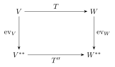
In the previous section we called $\operatorname{ev}_V \colon V \to V^{**}$ natural because it needs no choice, and promised a sharper sense: compatibility with every linear map. With dual maps available, we can state it. A linear map $T \colon V \to W$ has a dual $T' \colon W^{*} \to V^{*}$ , and that has a dual in turn, $T'' \mathrel{:=} (T')' \colon V^{**} \to W^{**},$ which points forward again, because we reversed twice.

Theorem 5.4.6 (The Evaluation Map Is Natural)

Let $V$ and $W$ be vector spaces over $F$ , and let $T \in \mathcal{L}(V, W)$ . Then $T''\,\operatorname{ev}_V = \operatorname{ev}_W\,T .$ That is, $T''(\operatorname{ev}_{\mathbf{v}}) = \operatorname{ev}_{T\mathbf{v}}$ for every $\mathbf{v} \in V$ . If $V$ and $W$ are finite-dimensional, then $T'' = \operatorname{ev}_W\,T\,\operatorname{ev}_V^{-1}$ .

The statement says that the square below commutes, for every linear map $T$ : going right then down (apply $T$ , then evaluate) equals going down then right (evaluate, then apply $T''$ ).

Diagram. Labels: T, T'', operatorname ev_V, operatorname ev_W, V, W, V^**, W^**

Proof. Let $\mathbf{v} \in V$ . Both $T''(\operatorname{ev}_{\mathbf{v}})$ and $\operatorname{ev}_{T\mathbf{v}}$ are functionals on $W^{*}$ , so let $\psi \in W^{*}$ . By Definition 5.4.1 applied to $T'$ , then to $T$ , $\bigl(T''(\operatorname{ev}_{\mathbf{v}})\bigr)(\psi) = \operatorname{ev}_{\mathbf{v}}(T'\psi) = (T'\psi)(\mathbf{v}) = \psi(T\mathbf{v}) = \operatorname{ev}_{T\mathbf{v}}(\psi).$ Hence $T''(\operatorname{ev}_{\mathbf{v}}) = \operatorname{ev}_{T\mathbf{v}}$ for every $\mathbf{v}$ , which is $T''\operatorname{ev}_V = \operatorname{ev}_W T$ . If $V$ is finite-dimensional, $\operatorname{ev}_V$ is an isomorphism (Theorem 5.3.2); composing on the right with $\operatorname{ev}_V^{-1}$ gives $T'' = \operatorname{ev}_W T\operatorname{ev}_V^{-1}$ .

So, once $V$ is identified with $V^{**}$ and $W$ with $W^{**}$ through evaluation, the double dual map $T''$ is $T$ . The matrices agree: by Theorem 5.3.2, $\operatorname{ev}$ carries $\mathcal{B}$ and $\mathcal{C}$ to the dual bases $\mathcal{B}^{**}$ and $\mathcal{C}^{**}$ of $\mathcal{B}^{*}$ and $\mathcal{C}^{*}$ , and two applications of Theorem 5.4.2 give $[T'']_{\mathcal{B}^{**}}^{\mathcal{C}^{**}} = \bigl(([T]_{\mathcal{B}}^{\mathcal{C}})^{\top}\bigr)^{\top} = [T]_{\mathcal{B}}^{\mathcal{C}}$ (Theorem 0.9.5). The rule $(\mathbf{A}^{\top})^{\top} = \mathbf{A}$ is the matrix form of naturality.

Remark. No such statement holds for $V \cong V^{*}$ . Suppose that for every finite-dimensional real space $V$ we had an isomorphism $\theta_V \colon V \to V^{*}$ , compatible with isomorphisms in the only way the directions allow: $\theta_V = T'\,\theta_W\,T$ for every isomorphism $T \colon V \to W$ . Take $V = W = \mathbb{R}$ and $T = 2\operatorname{id}$ . Then $T' = 2\operatorname{id}$ by Theorem 5.4.1 (a) and (c), so $\theta_{\mathbb{R}} = 2 \cdot 2 \cdot \theta_{\mathbb{R}} = 4\theta_{\mathbb{R}}$ , which forces $\theta_{\mathbb{R}} = 0$ , not an isomorphism. The dual space is isomorphic to $V$ , but not naturally.

5.4.5. Exercises

A. Check your understanding

Exercise (A1)

(a) Define the dual map $T'$ of $T \in \mathcal{L}(V, W)$ , including its domain and codomain.
(b) State the relation between $[T']_{\mathcal{C}^{*}}^{\mathcal{B}^{*}}$ and $[T]_{\mathcal{B}}^{\mathcal{C}}$ , with its hypotheses.
(c) True or false: $(ST)' = S'T'$ whenever $ST$ is defined. Justify your answer.
(d) True or false: $\operatorname{ker} T' = (\operatorname{ker} T)^{0}$ for every linear map between finite-dimensional spaces. Justify your answer.
(e) True or false: for $T \in \mathcal{L}(\mathbb{R}^4, \mathbb{R}^3)$ , the dual map $T'$ is never surjective. Justify your answer.
(f) Name the two tools combined to prove $\operatorname{rank} T' = \operatorname{rank} T$ .

Solution.

(a) For $T \colon V \to W$ , $T' \colon W^{*} \to V^{*}$ , $T'(\psi) = \psi T$ (Definition 5.4.1).
(b) If $V, W$ are finite-dimensional with bases $\mathcal{B}, \mathcal{C}$ and dual bases $\mathcal{B}^{*}, \mathcal{C}^{*}$ , then $[T']_{\mathcal{C}^{*}}^{\mathcal{B}^{*}} = ([T]_{\mathcal{B}}^{\mathcal{C}})^{\top}$ (Theorem 5.4.2).
(c) False. The correct rule is $(ST)' = T'S'$ (Theorem 5.4.1 (b)); for $T \colon U \to V$ , $S \colon V \to W$ with $U \neq W$ , the composite $S'T'$ is not even defined.
(d) False. $\operatorname{ker} T' = (\operatorname{im} T)^{0}$ . For the zero map $T \colon \mathbb{R} \to \mathbb{R}$ , $\operatorname{ker} T = \mathbb{R}$ , so $(\operatorname{ker} T)^{0} = \{0\}$ , while $T' = 0$ has kernel $\mathbb{R}^{*} \neq \{0\}$ .
(e) True. $T'$ maps $(\mathbb{R}^3)^{*}$ , of dimension $3$ , to $(\mathbb{R}^4)^{*}$ , of dimension $4$ , so it cannot be surjective (Corollary 2.3.2 (d)). This matches Corollary 5.4.5: $T$ cannot be injective.
(f) The Rank–Nullity Theorem (Theorem 2.3.1) and the dimension formula for annihilators, $\dim U + \dim U^{0} = \dim V$ (Theorem 5.2.2), together with $\operatorname{ker} T' = (\operatorname{im} T)^{0}$ .

B. Practice

Exercise (B1: Differentiation in dual bases)

Let $D \colon \mathbb{R}[x]_{\le 2} \to \mathbb{R}[x]_{\le 2}$ , $D(p) = p'$ , and let $\mathcal{B} = (1, x, x^2)$ with dual basis $\mathcal{B}^{*} = (\varphi_0, \varphi_1, \varphi_2)$ , $\varphi_k(p) =$ the coefficient of $x^k$ in $p$ . Compute $D'\varphi_0$ , $D'\varphi_1$ , $D'\varphi_2$ directly, write down $[D']_{\mathcal{B}^{*}}^{\mathcal{B}^{*}}$ , and check that it is $([D]_{\mathcal{B}}^{\mathcal{B}})^{\top}$ . Hence describe $\operatorname{ker} D'$ and $\operatorname{im} D'$ , and verify Theorem 5.4.3.

Solution. Let $p = a + bx + cx^2$ , so $Dp = b + 2cx$ . Then $(D'\varphi_0)(p) = \varphi_0(Dp) = b$ , $(D'\varphi_1)(p) = 2c$ , $(D'\varphi_2)(p) = 0$ . Hence $D'\varphi_0 = \varphi_1, \qquad D'\varphi_1 = 2\varphi_2, \qquad D'\varphi_2 = 0 .$ The coordinate vectors $(0, 1, 0)$ , $(0, 0, 2)$ , $(0, 0, 0)$ are the columns of $[D']_{\mathcal{B}^{*}}^{\mathcal{B}^{*}}$ . On the other side, $D(1) = 0$ , $D(x) = 1$ , $D(x^2) = 2x$ , so $[D]_{\mathcal{B}}^{\mathcal{B}} = \begin{pmatrix} 0 & 1 & 0 \\ 0 & 0 & 2 \\ 0 & 0 & 0 \end{pmatrix}, \qquad [D']_{\mathcal{B}^{*}}^{\mathcal{B}^{*}} = \begin{pmatrix} 0 & 0 & 0 \\ 1 & 0 & 0 \\ 0 & 2 & 0 \end{pmatrix} = ([D]_{\mathcal{B}}^{\mathcal{B}})^{\top},$ as Theorem 5.4.2 predicts.

From the formulas, $D'(c_0\varphi_0 + c_1\varphi_1 + c_2\varphi_2) = c_0\varphi_1 + 2c_1\varphi_2$ , which is $0$ iff $c_0 = c_1 = 0$ . So $\operatorname{ker} D' = \operatorname{span}(\varphi_2)$ and $\operatorname{im} D' = \operatorname{span}(\varphi_1, \varphi_2)$ . On the other hand $\operatorname{im} D = \mathbb{R}[x]_{\le 1} = \operatorname{span}(1, x)$ , and $\varphi_2$ is exactly the functional (up to scalars) vanishing on it, since $c_0\varphi_0 + c_1\varphi_1 + c_2\varphi_2$ kills $1$ and $x$ iff $c_0 = c_1 = 0$ . So $\operatorname{ker} D' = (\operatorname{im} D)^{0}$ . Also $\operatorname{ker} D = \operatorname{span}(1)$ , and a functional kills $1$ iff $c_0 = 0$ , so $(\operatorname{ker} D)^{0} = \operatorname{span}(\varphi_1, \varphi_2) = \operatorname{im} D'$ .

Exercise (B2: Kernel and image of a dual map)

Let $\mathbf{A} = \begin{pmatrix} 1 & 2 & -1 \\ -2 & -4 & 2 \end{pmatrix}$ and $T = T_{\mathbf{A}} \colon \mathbb{R}^3 \to \mathbb{R}^2$ . Find bases of $\operatorname{ker} T'$ and $\operatorname{im} T'$ as explicit functionals, and verify $\dim \operatorname{ker} T' + \dim \operatorname{im} T' = 2$ and $\operatorname{rank} T' = \operatorname{rank} T$ .

Solution. The second row is $-2$ times the first, so $\operatorname{rank} \mathbf{A} = 1$ , $\operatorname{im} T = \operatorname{col}(\mathbf{A}) = \operatorname{span}\bigl((1, -2)\bigr)$ , and $\operatorname{ker} T = \{ (x, y, z) : x + 2y - z = 0 \}$ , of dimension $2$ .

Kernel of $T'$ . As in Example (Kernel and Image of a Dual Map), $\psi(u, v) = b_1u + b_2v$ lies in $\operatorname{ker} T'$ iff $\mathbf{A}^{\top}\mathbf{b} = \mathbf{0}$ , that is, $b_1 - 2b_2 = 0$ , $2b_1 - 4b_2 = 0$ , $-b_1 + 2b_2 = 0$ . So $\mathbf{b} = t(2, 1)$ , and $\operatorname{ker} T' = \operatorname{span}(\psi_0)$ with $\psi_0(u, v) = 2u + v$ . Check: $\psi_0(1, -2) = 0$ , so $\psi_0 \in (\operatorname{im} T)^{0}$ , which has dimension $2 - 1 = 1$ .

Image of $T'$ . By Example (Dual Maps in Four Settings) (a), $\operatorname{im} T'$ is spanned by the rows of $\mathbf{A}$ read as functionals, $x + 2y - z$ and $-2x - 4y + 2z$ . The second is $-2$ times the first, so $\operatorname{im} T' = \operatorname{span}(\varphi_0)$ with $\varphi_0(x, y, z) = x + 2y - z$ . Check: $\varphi_0$ vanishes on $\operatorname{ker} T$ by the description of $\operatorname{ker} T$ , and $\dim (\operatorname{ker} T)^{0} = 3 - 2 = 1$ .

Hence $\dim \operatorname{ker} T' + \dim \operatorname{im} T' = 1 + 1 = 2 = \dim (\mathbb{R}^2)^{*}$ , and $\operatorname{rank} T' = 1 = \operatorname{rank} T$ .

Exercise (B3: The transpose of a product, again)

Let $\mathbf{A} \in M_{m \times n}(F)$ and $\mathbf{B} \in M_{n \times p}(F)$ . Using $T_{\mathbf{A}}T_{\mathbf{B}} = T_{\mathbf{A}\mathbf{B}}$ (Chapter 4, §01), Theorem 5.4.1 (b) and Theorem 5.4.2, give a new proof that $(\mathbf{A}\mathbf{B})^{\top} = \mathbf{B}^{\top} \mathbf{A}^{\top}$ .

Solution. Let $\mathcal{E}_p, \mathcal{E}_n, \mathcal{E}_m$ be the standard bases, with dual bases $\mathcal{E}_p^{*}, \mathcal{E}_n^{*}, \mathcal{E}_m^{*}$ . By Example (Matrix Maps and the Identity) (a), $[T_{\mathbf{A}}]_{\mathcal{E}_n}^{\mathcal{E}_m} = \mathbf{A}$ , $[T_{\mathbf{B}}]_{\mathcal{E}_p}^{\mathcal{E}_n} = \mathbf{B}$ , and $[T_{\mathbf{A}\mathbf{B}}]_{\mathcal{E}_p}^{\mathcal{E}_m} = \mathbf{A}\mathbf{B}$ . Since $T_{\mathbf{A}\mathbf{B}} = T_{\mathbf{A}}T_{\mathbf{B}}$ , Theorem 5.4.1 (b) gives $T_{\mathbf{A}\mathbf{B}}' = T_{\mathbf{B}}'T_{\mathbf{A}}'$ . Taking matrices, with Theorem 4.1.2 in the middle and Theorem 5.4.2 on the outside, $(\mathbf{A}\mathbf{B})^{\top} = [T_{\mathbf{A}\mathbf{B}}']_{\mathcal{E}_m^{*}}^{\mathcal{E}_p^{*}} = [T_{\mathbf{B}}'T_{\mathbf{A}}']_{\mathcal{E}_m^{*}}^{\mathcal{E}_p^{*}} = [T_{\mathbf{B}}']_{\mathcal{E}_n^{*}}^{\mathcal{E}_p^{*}}\,[T_{\mathbf{A}}']_{\mathcal{E}_m^{*}}^{\mathcal{E}_n^{*}} = \mathbf{B}^{\top} \mathbf{A}^{\top} .$ The reversal of order is now explained: it is the reversal of arrows under duality.

C. Going deeper

Exercise (C1: The Fredholm alternative)

(a) Let $V, W$ be finite-dimensional, $T \in \mathcal{L}(V, W)$ and $\mathbf{w} \in W$ . Prove that $T\mathbf{v} = \mathbf{w}$ has a solution $\mathbf{v} \in V$ if and only if $\psi(\mathbf{w}) = 0$ for every $\psi \in \operatorname{ker} T'$ .
(b) Deduce: for $\mathbf{A} \in M_{m \times n}(F)$ and $\mathbf{b} \in F^m$ , the system $\mathbf{A}\mathbf{x} = \mathbf{b}$ is consistent if and only if $\mathbf{y}^{\top}\mathbf{b} = 0$ for every $\mathbf{y} \in F^m$ with $\mathbf{A}^{\top}\mathbf{y} = \mathbf{0}$ .
(c) Let $\mathbf{A} = \begin{pmatrix} 1 & 1 \\ 1 & 2 \\ 1 & 3 \end{pmatrix}$ . Find a single linear condition on $\mathbf{b} = (b_1, b_2, b_3) \in \mathbb{R}^3$ that is equivalent to consistency of $\mathbf{A}\mathbf{x} = \mathbf{b}$ .

Hint: for (a), combine Theorem 5.4.3 with the description of a subspace by its annihilator in the previous section.

Solution.

(a) $T\mathbf{v} = \mathbf{w}$ has a solution iff $\mathbf{w} \in \operatorname{im} T$ . By Theorem 5.4.3 (a), $\operatorname{ker} T' = (\operatorname{im} T)^{0}$ . By Corollary 5.3.4 applied to the subspace $\operatorname{im} T$ of the finite-dimensional space $W$ , $\begin{aligned} \operatorname{im} T &= \{ \mathbf{w} \in W : \psi(\mathbf{w}) = 0 \text{ for every } \psi \in (\operatorname{im} T)^{0} \} \\ &= \{ \mathbf{w} \in W : \psi(\mathbf{w}) = 0 \text{ for every } \psi \in \operatorname{ker} T' \}. \end{aligned}$ This is the claim.
(b) Apply (a) to $T_{\mathbf{A}} \colon F^n \to F^m$ . By Theorem 5.1.1, every $\psi \in (F^m)^{*}$ is $\psi(\mathbf{u}) = \mathbf{y}^{\top}\mathbf{u}$ for a unique $\mathbf{y} \in F^m$ . By Example (Dual Maps in Four Settings) (a), $T_{\mathbf{A}}'\psi$ is represented by $\mathbf{A}^{\top}\mathbf{y}$ , and the zero functional by $\mathbf{0}$ ; by uniqueness of the representing vector, $\psi \in \operatorname{ker} T_{\mathbf{A}}'$ iff $\mathbf{A}^{\top}\mathbf{y} = \mathbf{0}$ . For such $\psi$ , $\psi(\mathbf{b}) = \mathbf{y}^{\top}\mathbf{b}$ . So (a) says: $\mathbf{A}\mathbf{x} = \mathbf{b}$ is consistent iff $\mathbf{y}^{\top}\mathbf{b} = 0$ for every $\mathbf{y}$ with $\mathbf{A}^{\top}\mathbf{y} = \mathbf{0}$ .
(c) $\mathbf{A}^{\top}\mathbf{y} = \mathbf{0}$ reads $y_1 + y_2 + y_3 = 0$ and $y_1 + 2y_2 + 3y_3 = 0$ . Subtracting, $y_2 + 2y_3 = 0$ , so $\mathbf{y} = t(1, -2, 1)$ . By (b), $\mathbf{A}\mathbf{x} = \mathbf{b}$ is consistent iff $\mathbf{y}^{\top}\mathbf{b} = 0$ for all these $\mathbf{y}$ , that is, iff $b_1 - 2b_2 + b_3 = 0 .$ In words, the system $x_1 + kx_2 = b_k$ ( $k = 1, 2, 3$ ) asks for a line through the points $(1, b_1), (2, b_2), (3, b_3)$ , and it exists exactly when the second difference $b_3 - 2b_2 + b_1$ vanishes. No inner product was used: $\mathbf{y}^{\top}\mathbf{b}$ is just a functional applied to $\mathbf{b}$ .

Exercise (C2: Invariant subspaces and annihilators)

Let $V$ be finite-dimensional, $T \in \mathcal{L}(V)$ , and $U$ a subspace of $V$ . Recall that $U$ is $T$ -invariant if $T\mathbf{u} \in U$ for every $\mathbf{u} \in U$ . Prove that $U$ is $T$ -invariant if and only if $U^{0}$ is $T'$ -invariant.

Solution. $(\Rightarrow)$ Suppose $U$ is $T$ -invariant, and let $\varphi \in U^{0}$ . For every $\mathbf{u} \in U$ , $(T'\varphi)(\mathbf{u}) = \varphi(T\mathbf{u}) = 0$ , because $T\mathbf{u} \in U$ . Hence $T'\varphi \in U^{0}$ , and $U^{0}$ is $T'$ -invariant.

$(\Leftarrow)$ Suppose $U^{0}$ is $T'$ -invariant, and let $\mathbf{u} \in U$ . For every $\varphi \in U^{0}$ , $T'\varphi \in U^{0}$ , so $\varphi(T\mathbf{u}) = (T'\varphi)(\mathbf{u}) = 0$ . Thus $T\mathbf{u}$ is killed by every functional in $U^{0}$ . By Corollary 5.3.4, $T\mathbf{u} \in U$ . Hence $U$ is $T$ -invariant.

Exercise (C3: Duality without finite dimension)

Let $V$ and $W$ be arbitrary vector spaces over $F$ , and $T \in \mathcal{L}(V, W)$ .

(a) Prove that if $T$ is surjective, then $T'$ is injective.
(b) Prove that if $T$ is injective, then $T'$ is surjective.
(c) Check (b) on $S \colon F[x] \to F[x]$ , $S(p) = xp$ , from Example (Dual Maps in Four Settings) (c): given $\varphi \in F[x]^{*}$ , find $\psi$ with $S'\psi = \varphi$ . Is $S'$ injective?

Hint: for (b), use Theorem 1.8.2 in $W$ .

Solution.

(a) By Theorem 5.4.3 (a), which needs no finite dimension, $\operatorname{ker} T' = (\operatorname{im} T)^{0} = W^{0}$ . A functional vanishing on all of $W$ is the zero functional, so $\operatorname{ker} T' = \{0\}$ and $T'$ is injective (Theorem 2.2.3).
(b) Let $\varphi \in V^{*}$ . By Theorem 1.8.3, $V$ has a basis $B$ . Since $T$ is injective, $T$ is one-to-one on $B$ , and $T(B)$ is linearly independent: a finite combination $\sum c_i T\mathbf{b}_i = T(\sum c_i\mathbf{b}_i) = \mathbf{0}$ with distinct $\mathbf{b}_i$ forces $\sum c_i\mathbf{b}_i = \mathbf{0}$ (Theorem 2.2.3), hence all $c_i = 0$ . By Theorem 1.8.2 there is a basis $C \supseteq T(B)$ of $W$ . By Theorem 2.1.6, there is $\psi \in W^{*}$ with $\psi(T\mathbf{b}) = \varphi(\mathbf{b})$ for $\mathbf{b} \in B$ , and $\psi(\mathbf{c}) = 0$ for $\mathbf{c} \in C \setminus T(B)$ ; this is well defined because each element of $T(B)$ is $T\mathbf{b}$ for exactly one $\mathbf{b}$ . Then $\psi T$ and $\varphi$ are linear and agree on the basis $B$ , so $T'\psi = \psi T = \varphi$ by the uniqueness part of Theorem 2.1.6. Hence $T'$ is surjective.
(c) Here $B = \{1, x, x^2, \dots\}$ and $S(B) = \{x, x^2, \dots\}$ , extended to a basis by adding $1$ . The recipe gives $\psi(x^{k+1}) = \varphi(x^k)$ for $k \ge 0$ and $\psi(1) = 0$ . Then $(S'\psi)(x^k) = \psi(x^{k+1}) = \varphi(x^k)$ , so $S'\psi = \varphi$ . The dual map $S'$ is not injective: $S'\varphi_0 = 0$ by Example (Dual Maps in Four Settings) (c). This matches the contrapositive of (a): $S$ is not surjective, since $1 \notin \operatorname{im} S$ , and indeed $\varphi_0$ is a non-zero functional vanishing on $\operatorname{im} S$ .