17.1 The Rayleigh Quotient

Chapter 13 used the number $\langle \mathbf{A}\mathbf{x}, \mathbf{x} \rangle$ as a test: positive for every non-zero $\mathbf{x}$ means positive definite, non-negative means positive semidefinite, and that was the end of it. Chapter 13 §05 then noticed that the test carries more information than the verdict — normalized, it ranges over the interval between the smallest and largest eigenvalues — and stopped there. This section makes the normalized quantity an object with a name, finds its range exactly, finds the vectors where it is flat, and extracts a first description of every eigenvalue as a maximum. The description is correct and unsatisfying, and saying precisely why is the business of §02.

Throughout, $F$ is $\mathbb{R}$ or $\mathbb{C}$ , every matrix is Hermitian, and its eigenvalues are indexed decreasingly, $\lambda_1(\mathbf{A}) \ge \dots \ge \lambda_n(\mathbf{A})$ , repeated according to multiplicity. The indexing presupposes that the eigenvalues are real, which is Theorem 12.2.1. Inner products are the standard ones of $F^n$ , linear in the first slot.

17.1.1. From a test to an object

Look at what Lemma 13.5.2 actually says. For a unit vector $\mathbf{x}$ , the number $\langle \mathbf{A}\mathbf{x}, \mathbf{x} \rangle$ lies between $\lambda_n(\mathbf{A})$ and $\lambda_1(\mathbf{A})$ , and it reaches both ends. The restriction to unit vectors is a nuisance: doubling $\mathbf{x}$ quadruples $\langle \mathbf{A}\mathbf{x}, \mathbf{x} \rangle$ , so for $\mathbf{A} \ne 0$ the raw quantity has no bounded range at all and every statement about it must carry the clause “for $\left\| \mathbf{x} \right\| = 1$ ” along. Dividing by $\left\| \mathbf{x} \right\|^2$ removes the nuisance permanently, and the resulting expression occurs often enough in what follows to deserve a name of its own.

The Rayleigh quotient measures how much a Hermitian matrix stretches a vector along its own direction, on a scale where the vector’s length has been divided out.

Definition 17.1.1 (Rayleigh Quotient)

Let $F$ be $\mathbb{R}$ or $\mathbb{C}$ and let $\mathbf{A} \in M_n(F)$ be Hermitian. The Rayleigh quotient of $\mathbf{A}$ is the function $R_{\mathbf{A}}(\mathbf{x}) \mathrel{:=} \frac{\langle \mathbf{A}\mathbf{x}, \mathbf{x} \rangle}{\langle \mathbf{x}, \mathbf{x} \rangle} ,$ defined at every $\mathbf{x} \in F^n$ with $\mathbf{x} \ne \mathbf{0}$ , and at no other vector.

For a self-adjoint operator $T$ on a finite-dimensional inner product space $V$ over $F$ , the same formula $R_T(\mathbf{v}) = \langle T\mathbf{v}, \mathbf{v} \rangle/\langle \mathbf{v}, \mathbf{v} \rangle$ , for $\mathbf{v} \ne \mathbf{0}$ , defines the Rayleigh quotient of $T$ .

Clause by clause. The word Hermitian is what makes the values real, and so what makes it sensible to ask for a maximum: by Proposition 11.6.7 (a), $\langle \mathbf{A}\mathbf{x}, \mathbf{x} \rangle \in \mathbb{R}$ for every $\mathbf{x}$ , even over $\mathbb{C}$ . The condition $\mathbf{x} \ne \mathbf{0}$ is what makes the fraction mean anything: $\langle \mathbf{x}, \mathbf{x} \rangle = \left\| \mathbf{x} \right\|^2 > 0$ exactly for $\mathbf{x} \ne \mathbf{0}$ , by positive definiteness of the inner product (Definition 11.1.1), and there is no value to assign at $\mathbf{0}$ — the numerator vanishes there too, and the quotient $0/0$ would have to be given a value by hand, which no theorem below would thank us for. So $R_{\mathbf{A}}$ is a real-valued function on $F^n \setminus \{\mathbf{0}\}$ .

Well-definedness has a second half, and it is the useful one. For a scalar $c \ne 0$ , $\begin{aligned} \langle \mathbf{A}(c\mathbf{x}), c\mathbf{x} \rangle &= c\,\overline{c}\,\langle \mathbf{A}\mathbf{x}, \mathbf{x} \rangle = \lvert c\rvert^2\langle \mathbf{A}\mathbf{x}, \mathbf{x} \rangle ,\\ \langle c\mathbf{x}, c\mathbf{x} \rangle &= \lvert c\rvert^2 \langle \mathbf{x}, \mathbf{x} \rangle , \end{aligned}$ so the factor $\lvert c\rvert^2$ cancels and $R_{\mathbf{A}}(c\mathbf{x}) = R_{\mathbf{A}}(\mathbf{x}) \qquad \text{for every } c \ne 0 .$ The Rayleigh quotient is therefore constant on each line through the origin with the origin removed. It is really a function on the set of lines, and the cheapest way to evaluate it is to normalize: for a unit vector $\mathbf{x}$ , $R_{\mathbf{A}}(\mathbf{x}) = \langle \mathbf{A}\mathbf{x}, \mathbf{x} \rangle .$ Every statement below may be read either way — over all non-zero vectors, or over the unit sphere — and we shall move between the two without comment.

Example (A diagonal matrix, and the whole chapter in miniature)

Let $\mathbf{A} = \operatorname{diag}(d_1, \dots, d_n)$ with real $d_i$ . Compute $R_{\mathbf{A}}$ .

Solution. For $\mathbf{x} = (x_1, \dots, x_n) \ne \mathbf{0}$ we have $\mathbf{A}\mathbf{x} = (d_1x_1, \dots, d_nx_n)$ , so $R_{\mathbf{A}}(\mathbf{x}) = \frac{\sum_{i} d_i\lvert x_i\rvert^2}{\sum_i \lvert x_i\rvert^2} = \sum_{i} w_i d_i , \qquad w_i = \frac{\lvert x_i\rvert^2}{\left\| \mathbf{x} \right\|^2} .$ The weights $w_i$ are non-negative and sum to $1$ . So $R_{\mathbf{A}}(\mathbf{x})$ is a weighted average of the diagonal entries, and $\mathbf{x}$ is nothing but the recipe for the weights.

That one line is the entire chapter in miniature, and it is worth pausing on. A weighted average of $d_1, \dots, d_n$ can be any number between the smallest and the largest, and nothing else; it equals the largest only when all the weight sits on the largest entries; and to force it down to the second largest one must forbid the weight from sitting on the first. Every theorem in this chapter is one of those three sentences, stated for a general Hermitian matrix, where the diagonal entries are replaced by the eigenvalues and the coordinates $x_i$ by the coefficients of $\mathbf{x}$ in an orthonormal eigenbasis. The spectral theorem is what turns the general case into this one.

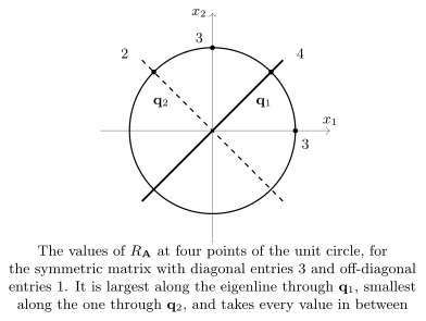
Example (A symmetric matrix on the unit circle)

Let $\mathbf{A} = \begin{pmatrix} 3 & 1 \\ 1 & 3\end{pmatrix} \in M_2(\mathbb{R})$ . Describe $R_{\mathbf{A}}$ on the unit circle, and find its largest and smallest values.

Solution. The eigenvalues are $4$ and $2$ , with orthogonal eigenvectors $\mathbf{q}_1 = \tfrac{1}{\sqrt2}(1,1)$ and $\mathbf{q}_2 = \tfrac1{\sqrt2}(1,-1)$ : indeed $\mathbf{A}(1,1) = (4,4)$ and $\mathbf{A}(1,-1) = (2,-2)$ . Writing a unit vector as $\mathbf{x} = (\cos\theta, \sin\theta)$ , $R_{\mathbf{A}}(\mathbf{x}) = \langle \mathbf{A}\mathbf{x}, \mathbf{x} \rangle = 3\cos^2\theta + 2\cos\theta\sin\theta + 3\sin^2\theta = 3 + \sin 2\theta .$ So the values run over $[2, 4]$ ; the maximum $4$ occurs at $\theta = \pi/4$ and $\theta = 5\pi/4$ , that is along the line through $\mathbf{q}_1$ , and the minimum $2$ at $\theta = 3\pi/4$ and $7\pi/4$ , along the line through $\mathbf{q}_2$ . At $\theta = 0$ and $\theta = \pi/2$ the value is $3$ , the average of the two eigenvalues, which is also $a_{11} = a_{22}$ .

$Diagram. Labels: x_1, x_2, 4, 2, 3, mathbf q_1, mathbf q_2, The values of R_mathbf A at four points of the unit circle, for\\ the symmetric matrix with diagonal entries 3 and off-diagonal\\ entries 1. It is largest along the eigenline through mathbf q_1, smallest\\ along the one through mathbf q_2, and takes every value in between$

Example (Two matrices whose quotient is forced)

Two further cases, at opposite extremes.

(a) The identity. $R_{\mathbf{I}}(\mathbf{x}) = \langle \mathbf{x}, \mathbf{x} \rangle/\langle \mathbf{x}, \mathbf{x} \rangle = 1$ for every $\mathbf{x} \ne \mathbf{0}$ . The quotient is constant, and the constant is the only eigenvalue. More generally $R_{c\mathbf{I}} \equiv c$ for real $c$ .
(b) An orthogonal projection. Let $\mathbf{P} \in M_n(F)$ be the matrix of the orthogonal projection onto a subspace $U$ , so $\mathbf{P}^2 = \mathbf{P}$ and $\mathbf{P}^{*} = \mathbf{P}$ (Theorem 13.12.1). Then $\langle \mathbf{P}\mathbf{x}, \mathbf{x} \rangle = \langle \mathbf{P}^2\mathbf{x}, \mathbf{x} \rangle = \langle \mathbf{P}\mathbf{x}, \mathbf{P}\mathbf{x} \rangle = \left\| \mathbf{P}\mathbf{x} \right\|^2$ , so $R_{\mathbf{P}}(\mathbf{x}) = \frac{\left\| \mathbf{P}\mathbf{x} \right\|^2}{\left\| \mathbf{x} \right\|^2} \in [0, 1] ,$ the fraction of $\mathbf{x}$ that survives the projection. Since $\left\| \mathbf{x} \right\|^2 = \left\| \mathbf{P}\mathbf{x} \right\|^2 + \left\| \mathbf{x} - \mathbf{P}\mathbf{x} \right\|^2$ by Theorem 11.1.3, it equals $1$ exactly when $\mathbf{P}\mathbf{x} = \mathbf{x}$ , that is on $U \setminus\{\mathbf{0}\}$ , and $0$ exactly when $\mathbf{P}\mathbf{x} = \mathbf{0}$ , that is on $U^{\perp}\setminus\{\mathbf{0}\}$ — matching the eigenvalues $1$ and $0$ of $\mathbf{P}$ .

Case (a) is the degenerate one, and it earns its place: when all the eigenvalues coincide the interval of values collapses to a point, every non-zero vector is an eigenvector, and every theorem below becomes an equality between two copies of the same number. A statement that fails to survive $\mathbf{A} = c\mathbf{I}$ has been stated wrongly.

Example (Change one word: drop Hermitian)

Take $\mathbf{A} = \begin{pmatrix} 0 & 1 \\ 0 & 0\end{pmatrix} \in M_2(\mathbb{C})$ , which is not Hermitian, and form $\langle \mathbf{A}\mathbf{x}, \mathbf{x} \rangle/\langle \mathbf{x}, \mathbf{x} \rangle$ anyway. At $\mathbf{x} = (1, i)$ the numerator is $\langle (i, 0), (1,i) \rangle = i \cdot \overline{1} = i$ and the denominator is $2$ , so the quotient is $i/2$ , which is not real. The clause that fails is the word Hermitian in Definition 17.1.1, and it fails at the first step: Proposition 11.6.7 (a) is what made the numerator real, and its hypothesis is gone.

Over $\mathbb{R}$ the failure is quieter and worse. For $\mathbf{A} = \begin{pmatrix} 0 & -1 \\ 1 & 0\end{pmatrix} \in M_2(\mathbb{R})$ and real $\mathbf{x} = (x_1, x_2)$ , $\langle \mathbf{A}\mathbf{x}, \mathbf{x} \rangle = -x_2x_1 + x_1x_2 = 0 ,$ so the quotient is real, and identically $0$ . It is perfectly well behaved and tells us nothing: $\mathbf{A}$ has no real eigenvalue at all, and there is no interval $[\lambda_n, \lambda_1]$ for the quotient to describe.

Why this definition, then. Dropping “Hermitian” costs the reality of the values, hence any notion of largest; the real $2\times 2$ example above shows that it also destroys the link with the spectrum even when the values happen to stay real. Dropping the denominator costs scale invariance, and with it the possibility of writing $\max$ without a side condition. Keeping the denominator but allowing $\mathbf{x} = \mathbf{0}$ costs nothing but sense.

Warning. $R_{\mathbf{A}}(\mathbf{x})$ and $\langle \mathbf{A}\mathbf{x}, \mathbf{x} \rangle$ are the same number only for unit $\mathbf{x}$ . The bound $\langle \mathbf{A}\mathbf{x}, \mathbf{x} \rangle \le \lambda_1(\mathbf{A})$ of Lemma 13.5.2 is stated for unit vectors and is false without that hypothesis: for $\mathbf{A} = \mathbf{I}_2$ and $\mathbf{x} = (10, 0)$ it would read $100 \le 1$ . The bound $R_{\mathbf{A}}(\mathbf{x}) \le \lambda_1(\mathbf{A})$ , by contrast, holds for every $\mathbf{x} \ne \mathbf{0}$ . Whenever a maximum over “all $\mathbf{x}$ ” appears below, it is a maximum of the quotient; the un-normalized form of the same statement always carries $\left\| \mathbf{x} \right\| = 1$ with it.

17.1.2. What values it takes

Lemma 13.5.2 gives the two ends of the range. The following proposition adds that nothing in between is missing, which is a smaller statement than it looks and is worth proving explicitly rather than quoting a continuity argument.

Proposition 17.1.1 (The Range of the Rayleigh Quotient)

Let $\mathbf{A} \in M_n(F)$ be Hermitian, $n \ge 1$ . Then $\bigl\{ R_{\mathbf{A}}(\mathbf{x}) : \mathbf{x} \in F^n,\ \mathbf{x} \ne \mathbf{0} \bigr\} = \bigl[\lambda_n(\mathbf{A}),\ \lambda_1(\mathbf{A})\bigr] ,$ the whole closed interval. In particular $\lambda_1(\mathbf{A}) = \max_{\mathbf{x} \ne \mathbf{0}} R_{\mathbf{A}}(\mathbf{x}), \qquad \lambda_n(\mathbf{A}) = \min_{\mathbf{x} \ne \mathbf{0}} R_{\mathbf{A}}(\mathbf{x}) ,$ and both are attained, at unit eigenvectors for $\lambda_1(\mathbf{A})$ and $\lambda_n(\mathbf{A})$ .

Idea. Two inclusions of quite different weights. $(\subseteq)$ is Lemma 13.5.2 with the normalization divided out, and costs one line. $(\supseteq)$ asks for a vector realizing each intermediate value; the natural instinct is to move continuously along the sphere from a top eigenvector to a bottom one and quote the intermediate value theorem, but there is no need to import anything. Mixing a top eigenvector and a bottom eigenvector in the proportion $t : 1-t$ puts weight $t$ on $\lambda_1$ and $1-t$ on $\lambda_n$ , and the weighted average of Example (A diagonal matrix, and the whole chapter in miniature) sweeps the interval as $t$ does.

Proof. By the spectral theorem for matrices — Corollary 12.4.3 over $\mathbb{C}$ , Corollary 12.5.2 over $\mathbb{R}$ — there is an orthonormal basis $(\mathbf{q}_1, \dots, \mathbf{q}_n)$ of $F^n$ with $\mathbf{A}\mathbf{q}_i = \lambda_i(\mathbf{A})\mathbf{q}_i$ for every $i$ .

$(\subseteq)$ Let $\mathbf{x} \ne \mathbf{0}$ and put $\mathbf{u} = \mathbf{x}/\left\| \mathbf{x} \right\|$ , a unit vector. By the scale invariance established above, $R_{\mathbf{A}}(\mathbf{x}) = R_{\mathbf{A}}(\mathbf{u}) = \langle \mathbf{A}\mathbf{u}, \mathbf{u} \rangle$ , which lies in $[\lambda_n(\mathbf{A}), \lambda_1(\mathbf{A})]$ by Lemma 13.5.2.

$(\supseteq)$ Let $\mu \in [\lambda_n(\mathbf{A}), \lambda_1(\mathbf{A})]$ . If $\lambda_1(\mathbf{A}) = \lambda_n(\mathbf{A})$ the interval is the single point $\mu = \lambda_1(\mathbf{A}) = R_{\mathbf{A}}(\mathbf{q}_1)$ , and we are done. Otherwise put $t = \frac{\mu - \lambda_n(\mathbf{A})}{\lambda_1(\mathbf{A}) - \lambda_n(\mathbf{A})} \in [0, 1], \qquad \mathbf{x} = \sqrt{t}\,\mathbf{q}_1 + \sqrt{1-t}\,\mathbf{q}_n ,$ which is legitimate because the denominator is non-zero and both square roots are of non-negative reals. Note $n \ge 2$ here, since $\lambda_1 \ne \lambda_n$ , so $\mathbf{q}_1$ and $\mathbf{q}_n$ are distinct members of an orthonormal list. By Theorem 11.2.1 (c), $\left\| \mathbf{x} \right\|^2 = t + (1-t) = 1 ,$ so in particular $\mathbf{x} \ne \mathbf{0}$ . Since $\mathbf{A}\mathbf{x} = \sqrt t\,\lambda_1(\mathbf{A})\mathbf{q}_1 + \sqrt{1-t}\,\lambda_n(\mathbf{A})\mathbf{q}_n$ , Theorem 11.2.1 (b) gives $R_{\mathbf{A}}(\mathbf{x}) = \langle \mathbf{A}\mathbf{x}, \mathbf{x} \rangle = t\,\lambda_1(\mathbf{A}) + (1-t)\,\lambda_n(\mathbf{A}) = \mu ,$ the last equality by the choice of $t$ . So every point of the interval is a value.

For the attainment, $R_{\mathbf{A}}(\mathbf{q}_1) = \lambda_1(\mathbf{A})$ and $R_{\mathbf{A}}(\mathbf{q}_n) = \lambda_n(\mathbf{A})$ . This proves the proposition.

So the range is an interval, not a finite set, even though $\mathbf{A}$ has at most $n$ eigenvalues. That single fact is responsible for most of the confusion this chapter has to clear up, and the warning below spells out why.

Quick check. For $\mathbf{A} = \operatorname{diag}(6, 3, 0)$ , write down two unit vectors with Rayleigh quotient $4$ , each having one zero coordinate, in different positions.

Solution. Mixing $\mathbf{e}_1$ and $\mathbf{e}_3$ as in the proof: $4 = 6t + 0(1-t)$ gives $t = 2/3$ and $\mathbf{x} = \bigl(\sqrt{2/3},\, 0,\, \sqrt{1/3}\bigr)$ , for which $R_{\mathbf{A}}(\mathbf{x}) = 6\cdot\tfrac23 + 0\cdot\tfrac13 = 4$ . Mixing $\mathbf{e}_1$ and $\mathbf{e}_2$ instead: $4 = 6t + 3(1-t)$ gives $t = 1/3$ and $\mathbf{y} = \bigl(\sqrt{1/3},\, \sqrt{2/3},\, 0\bigr)$ , for which $R_{\mathbf{A}}(\mathbf{y}) = 6\cdot\tfrac13 + 3\cdot\tfrac23 = 4$ . A value of $R_{\mathbf{A}}$ is realized by many vectors, and they need not resemble each other.

17.1.3. Where the quotient is flat

The maximum and the minimum are attained at eigenvectors. There is a converse, and it identifies the eigenvectors among all vectors by a condition that does not mention eigenvalues: they are the places where $R_{\mathbf{A}}$ does not move to first order. Everything needed is one algebraic identity, exact for every $t$ , so no calculus enters.

Proposition 17.1.2 (Critical Points of the Rayleigh Quotient)

Let $\mathbf{A} \in M_n(F)$ be Hermitian, let $\mathbf{x} \in F^n$ be a unit vector and put $\mu = R_{\mathbf{A}}(\mathbf{x}) = \langle \mathbf{A}\mathbf{x}, \mathbf{x} \rangle$ . For every $\mathbf{v} \in F^n$ and every $t \in \mathbb{R}$ with $\mathbf{x} + t\mathbf{v} \ne \mathbf{0}$ ,

\begin{aligned} &R_{\mathbf{A}}(\mathbf{x} + t\mathbf{v}) - \mu \\ &\qquad = \frac{2t\operatorname{Re}\langle \mathbf{A}\mathbf{x} - \mu\mathbf{x}, \mathbf{v} \rangle + t^2\bigl(\langle \mathbf{A}\mathbf{v}, \mathbf{v} \rangle - \mu\left\| \mathbf{v} \right\|^2\bigr)}{\left\| \mathbf{x} + t\mathbf{v} \right\|^2} . \end{aligned}

(17.1.1)

Moreover:

(a) $\operatorname{Re}\langle \mathbf{A}\mathbf{x} - \mu\mathbf{x}, \mathbf{v} \rangle = 0$ for every $\mathbf{v} \in F^n$ if and only if $\mathbf{A}\mathbf{x} = \mu\mathbf{x}$ ; that is, if and only if $\mathbf{x}$ is an eigenvector of $\mathbf{A}$ , necessarily for the eigenvalue $\mu$ .
(b) If $R_{\mathbf{A}}(\mathbf{x}) \ge R_{\mathbf{A}}(\mathbf{y})$ for every $\mathbf{y} \ne \mathbf{0}$ , then the condition in (a) holds. The same is true if $R_{\mathbf{A}}(\mathbf{x}) \le R_{\mathbf{A}}(\mathbf{y})$ for every $\mathbf{y} \ne \mathbf{0}$ .

Idea. Expand the numerator and the denominator of $R_{\mathbf{A}}(\mathbf{x} + t\mathbf{v})$ in powers of $t$ and subtract $\mu$ times the denominator from the numerator. The constant terms cancel by the definition of $\mu$ , and what is left is exactly Eq. 17.1.1. The coefficient of $t$ is the object of interest: (a) says it vanishes in every direction precisely at eigenvectors, and (b) says that at a maximum it must vanish, since otherwise a small step in the right direction would increase the quotient — the $t^2$ term cannot interfere, because for small $t$ it is smaller than the $t$ term.

Proof. The identity. Expanding by sesquilinearity, $\begin{aligned} \langle \mathbf{A}(\mathbf{x} + t\mathbf{v}), \mathbf{x} + t\mathbf{v} \rangle &= \langle \mathbf{A}\mathbf{x}, \mathbf{x} \rangle + t\langle \mathbf{A}\mathbf{x}, \mathbf{v} \rangle + t\langle \mathbf{A}\mathbf{v}, \mathbf{x} \rangle + t^2\langle \mathbf{A}\mathbf{v}, \mathbf{v} \rangle \\ &= \mu + 2t\operatorname{Re}\langle \mathbf{A}\mathbf{x}, \mathbf{v} \rangle + t^2\langle \mathbf{A}\mathbf{v}, \mathbf{v} \rangle , \end{aligned}$ where the second line used $\langle \mathbf{A}\mathbf{v}, \mathbf{x} \rangle = \langle \mathbf{v}, \mathbf{A}\mathbf{x} \rangle = \overline{\langle \mathbf{A}\mathbf{x}, \mathbf{v} \rangle}$ , the first equality because $\mathbf{A}$ is Hermitian and the second by conjugate symmetry (Definition 11.1.1), together with $\langle \mathbf{A}\mathbf{x}, \mathbf{x} \rangle = \mu$ for the unit vector $\mathbf{x}$ . The same computation with $\mathbf{A}$ replaced by $\mathbf{I}$ , where the constant term is $\left\| \mathbf{x} \right\|^2 = 1$ , gives $\left\| \mathbf{x} + t\mathbf{v} \right\|^2 = 1 + 2t\operatorname{Re}\langle \mathbf{x}, \mathbf{v} \rangle + t^2\left\| \mathbf{v} \right\|^2 .$ Since $\mu$ is real, $\mu\operatorname{Re}\langle \mathbf{x}, \mathbf{v} \rangle = \operatorname{Re}\langle \mu\mathbf{x}, \mathbf{v} \rangle$ . Subtracting $\mu\left\| \mathbf{x}+t\mathbf{v} \right\|^2$ from the first display therefore leaves $2t\operatorname{Re}\langle \mathbf{A}\mathbf{x} - \mu\mathbf{x}, \mathbf{v} \rangle + t^2\bigl(\langle \mathbf{A}\mathbf{v}, \mathbf{v} \rangle - \mu\left\| \mathbf{v} \right\|^2\bigr) ,$ and dividing by $\left\| \mathbf{x} + t\mathbf{v} \right\|^2 \ne 0$ gives Eq. 17.1.1.

(a) Put $\mathbf{w} = \mathbf{A}\mathbf{x} - \mu\mathbf{x}$ . $(\Leftarrow)$ If $\mathbf{A}\mathbf{x} = \mu\mathbf{x}$ then $\mathbf{w} = \mathbf{0}$ and every $\langle \mathbf{w}, \mathbf{v} \rangle$ vanishes. $(\Rightarrow)$ Take $\mathbf{v} = \mathbf{w}$ : the hypothesis gives $\operatorname{Re}\langle \mathbf{w}, \mathbf{w} \rangle = \left\| \mathbf{w} \right\|^2 = 0$ , so $\mathbf{w} = \mathbf{0}$ by positive definiteness, that is $\mathbf{A}\mathbf{x} = \mu\mathbf{x}$ . Since $\mathbf{x} \ne \mathbf{0}$ , this exhibits $\mathbf{x}$ as an eigenvector for the eigenvalue $\mu$ .
(b) Suppose $\mathbf{x}$ maximizes $R_{\mathbf{A}}$ and, for a contradiction, that $c \mathrel{:=} 2\operatorname{Re}\langle \mathbf{A}\mathbf{x} - \mu\mathbf{x}, \mathbf{v} \rangle \ne 0$ for some $\mathbf{v}$ ; then $\mathbf{v} \ne \mathbf{0}$ . Put $d = \langle \mathbf{A}\mathbf{v}, \mathbf{v} \rangle - \mu\left\| \mathbf{v} \right\|^2$ , and let $t$ be any real number with $0 < \lvert t\rvert < \frac{1}{2\left\| \mathbf{v} \right\|}, \qquad \lvert t \rvert\,\lvert d\rvert < \tfrac12\lvert c\rvert , \qquad t \ \text{of the same sign as}\ c ,$ which is possible because the two upper bounds are positive. The first bound gives $\left\| \mathbf{x} + t\mathbf{v} \right\| \ge \left\| \mathbf{x} \right\| - \lvert t\rvert\left\| \mathbf{v} \right\| > 1 - \tfrac12 > 0$ , by the triangle inequality (Corollary 11.1.6), so $\mathbf{x} + t\mathbf{v} \ne \mathbf{0}$ and the identity applies. The second gives $\lvert td\rvert < \lvert c \rvert/2$ , so $c + td$ has the same sign as $c$ , and hence $t(c + td) > 0$ . By Eq. 17.1.1, $R_{\mathbf{A}}(\mathbf{x} + t\mathbf{v}) - \mu = \frac{t\,(c + t d)}{\left\| \mathbf{x}+t\mathbf{v} \right\|^2} > 0 ,$ contradicting the maximality of $R_{\mathbf{A}}(\mathbf{x})$ . So $c = 0$ for every $\mathbf{v}$ . For a minimizer, apply what has just been proved to $-\mathbf{A}$ , whose Rayleigh quotient is $-R_{\mathbf{A}}$ , so that a minimizer of $R_{\mathbf{A}}$ is a maximizer of $R_{-\mathbf{A}}$ ; the condition in (a) for $-\mathbf{A}$ and $-\mu$ is the same condition. This proves the proposition.

Call a unit vector $\mathbf{x}$ a critical point of $R_{\mathbf{A}}$ when the condition in (a) holds, that is, when the coefficient of $t$ in Eq. 17.1.1 vanishes in every direction $\mathbf{v}$ — when $R_{\mathbf{A}}$ moves away from $R_{\mathbf{A}}(\mathbf{x})$ only at second order. Parts (a) and (b) then say: the critical points of $R_{\mathbf{A}}$ on the unit sphere are exactly the unit eigenvectors of $\mathbf{A}$ , the critical values are exactly the eigenvalues, and every maximizer and every minimizer is among them. That the eigenvalues are all realized as critical values is a direct computation: $R_{\mathbf{A}}(\mathbf{q}_i) = \langle \lambda_i\mathbf{q}_i, \mathbf{q}_i \rangle = \lambda_i$ , and each $\mathbf{q}_i$ is a unit eigenvector, hence a critical point by (b).

Remark. A reader who knows calculus will recognize Eq. 17.1.1 as saying that the directional derivative of $R_{\mathbf{A}}$ at a unit vector $\mathbf{x}$ in the direction $\mathbf{v}$ is $2\operatorname{Re}\langle \mathbf{A}\mathbf{x} - \mu\mathbf{x}, \mathbf{v} \rangle$ , so that “critical point” has its usual meaning of a vanishing gradient. Nothing above uses derivatives: the identity Eq. 17.1.1 is exact for every $t$ , not an approximation, and the argument in (b) compares two explicit numbers. This matters for the accounting in the next remark.

Remark. The promise from Chapter 12 §02, and what it cost. Chapter 12 §02 proved that a real self-adjoint operator has an eigenvalue by an algebraic route, and then described the alternative it was declining: “the function $\mathbf{v} \mapsto \langle T\mathbf{v}, \mathbf{v} \rangle$ is real-valued and continuous on the unit sphere of $V$ , which is closed and bounded, so it attains a maximum, and a vector where it does so turns out to be an eigenvector for the largest eigenvalue. That argument is shorter to state but it is analysis, not algebra, and it needs the extreme value theorem; we keep to the algebraic route so that nothing in this chapter depends on it. The maximization picture returns in Chapter 17, where the Rayleigh quotient and the Courant–Fischer theorem describe every eigenvalue of a self-adjoint operator by optimization.”

The picture has now returned, and the account can be settled exactly. The clause “a vector where it does so turns out to be an eigenvector” is Proposition 17.1.2 (b) and (a), and that the eigenvalue is the largest one is Proposition 17.1.1; neither invokes an analytic fact. What Chapter 12 would have had to import is only the existence of the maximizer, which is the extreme value theorem — fact (A4) of Chapter 16’s introduction — applied to a continuous function on the unit sphere, compact by fact (A3). This chapter does not import it, because it does not have to: the spectral theorem is available here and it hands over the maximizer by name, namely $\mathbf{q}_1$ , in Proposition 17.1.1. So the optimization description of eigenvalues in this chapter is a consequence of the spectral theorem, not an independent proof of it. One honest qualification: the spectral theorem itself rests on the fundamental theorem of algebra (Theorem 6.5.1), which Chapter 6 §05 proved with the extreme value theorem on a disc. So the analysis is not absent from the foundations — it was spent once, there, and nothing here spends it again. Section 2 completes the promise for the intermediate eigenvalues, on the same terms.

17.1.4. Why the second eigenvalue is not a second maximum

Warning. $\lambda_2(\mathbf{A})$ is not “the second largest value of $R_{\mathbf{A}}$ ”, and there is no sense in which it could be. Take $\mathbf{A} = \operatorname{diag}(3, 1, -1)$ , so $\lambda_1 = 3$ , $\lambda_2 = 1$ , $\lambda_3 = -1$ . By Proposition 17.1.1 the set of values of $R_{\mathbf{A}}$ is the whole interval $[-1, 3]$ . Three things go wrong at once.

There is no second largest value. The values below $3$ form the interval $[-1, 3)$ , which has no largest element. So the phrase does not describe a number.
The value $\lambda_2$ is attained, but so is every other value, and not only at eigenvectors. At $\mathbf{x} = \tfrac1{\sqrt2}(1, 0, 1)$ the quotient is $\tfrac12(3) + \tfrac12(-1) = 1 = \lambda_2(\mathbf{A})$ , and $\mathbf{x}$ is not an eigenvector of $\mathbf{A}$ : it mixes the eigenvectors $\mathbf{e}_1$ and $\mathbf{e}_3$ of the first and the third eigenvalues, and $\lambda_2$ plays no part in it.
Removing a direction does not help by itself. At $\mathbf{y} = \tfrac1{\sqrt2}(1,1,0)$ , which is orthogonal to the eigenvector $\mathbf{e}_3$ of $\lambda_3$ , the quotient is $\tfrac12(3) + \tfrac12(1) = 2$ , strictly between $\lambda_1$ and $\lambda_2$ . Constraining $\mathbf{x}$ to a subspace changes the answer, and which subspace is everything.

Whatever describes $\lambda_2$ must be a maximum over something smaller than the sphere.

The last bullet says what to try. Cutting the sphere down by orthogonality to the top eigenvector does work, and the proof is Example (A diagonal matrix, and the whole chapter in miniature) again, with the top entry removed from the average.

Proposition 17.1.3 (Eigenvalues by Deflation)

Let $\mathbf{A} \in M_n(F)$ be Hermitian and let $(\mathbf{q}_1, \dots, \mathbf{q}_n)$ be an orthonormal basis of $F^n$ with $\mathbf{A}\mathbf{q}_i = \lambda_i(\mathbf{A})\mathbf{q}_i$ for every $i$ . Then for every $k$ with $1 \le k \le n$ , $\lambda_k(\mathbf{A}) = \max\bigl\{ R_{\mathbf{A}}(\mathbf{x}) : \mathbf{x} \ne \mathbf{0},\ \mathbf{x} \perp \mathbf{q}_1, \dots, \mathbf{q}_{k-1} \bigr\} ,$ the maximum being attained at $\mathbf{x} = \mathbf{q}_k$ . For $k = 1$ the list of constraints is empty and the statement is Proposition 17.1.1.

Idea. The constraints do one thing: they delete the first $k-1$ coordinates in the eigenbasis. What is left is the weighted average of Example (A diagonal matrix, and the whole chapter in miniature) over the remaining eigenvalues $\lambda_k \ge \dots \ge \lambda_n$ , whose largest member is $\lambda_k$ .

Proof. Let $W = \{\mathbf{x} \in F^n : \langle \mathbf{x}, \mathbf{q}_i \rangle = 0 \text{ for } 1 \le i \le k-1\}$ . By Theorem 11.2.1 (a) every $\mathbf{x} \in F^n$ satisfies $\mathbf{x} = \sum_{i=1}^{n}\langle \mathbf{x}, \mathbf{q}_i \rangle\mathbf{q}_i$ , so $\mathbf{x} \in W$ exactly when $\mathbf{x} \in \operatorname{span}(\mathbf{q}_k, \dots, \mathbf{q}_n)$ .

Let $\mathbf{x} \in W$ with $\mathbf{x} \ne \mathbf{0}$ , and write $c_i = \langle \mathbf{x}, \mathbf{q}_i \rangle$ , so that $\mathbf{x} = \sum_{i \ge k}c_i\mathbf{q}_i$ . Then $\mathbf{A}\mathbf{x} = \sum_{i\ge k}\lambda_i(\mathbf{A})c_i\mathbf{q}_i$ , and Theorem 11.2.1 (b), (c) give $\langle \mathbf{A}\mathbf{x}, \mathbf{x} \rangle = \sum_{i \ge k}\lambda_i(\mathbf{A})\lvert c_i\rvert^2 , \qquad \left\| \mathbf{x} \right\|^2 = \sum_{i\ge k}\lvert c_i\rvert^2 > 0 .$ Hence $R_{\mathbf{A}}(\mathbf{x})$ is a weighted average of $\lambda_k(\mathbf{A}), \dots, \lambda_n(\mathbf{A})$ with non-negative weights $\lvert c_i\rvert^2/\left\| \mathbf{x} \right\|^2$ summing to $1$ . The largest of those eigenvalues is $\lambda_k(\mathbf{A})$ , because the list is indexed decreasingly, so $R_{\mathbf{A}}(\mathbf{x}) \le \lambda_k(\mathbf{A})$ .

Finally $\mathbf{q}_k \in W$ , since the $\mathbf{q}_i$ are orthonormal, and $R_{\mathbf{A}}(\mathbf{q}_k) = \langle \lambda_k(\mathbf{A})\mathbf{q}_k, \mathbf{q}_k \rangle = \lambda_k(\mathbf{A})$ . So the bound is attained and the supremum is a maximum. This proves the proposition.

Quick check. In Proposition 17.1.3, does the value of the maximum depend on which orthonormal eigenbasis $(\mathbf{q}_1, \dots, \mathbf{q}_n)$ is chosen? Does the maximizing vector?

Solution. The value does not: it is $\lambda_k(\mathbf{A})$ , a number attached to $\mathbf{A}$ alone. The maximizing vector generally does, and so does the constraint set $W$ . For $\mathbf{A} = \operatorname{diag}(1, 1, 0)$ and $k = 2$ , one admissible eigenbasis is $(\mathbf{e}_1, \mathbf{e}_2, \mathbf{e}_3)$ , giving $W = \operatorname{span}(\mathbf{e}_2, \mathbf{e}_3)$ and maximizer $\mathbf{e}_2$ ; another is $\bigl(\tfrac1{\sqrt2}(1,1,0), \tfrac1{\sqrt2}(1,-1,0), \mathbf{e}_3\bigr)$ , giving a different $W$ and the maximizer $\tfrac1{\sqrt2}(1,-1,0)$ . Both maxima equal $\lambda_2(\mathbf{A}) = 1$ .

17.1.5. What is still wrong

Proposition 17.1.3 is a complete answer to the question “what is $\lambda_k(\mathbf{A})$ , as an optimization?” and it is nearly useless. The reason is visible in its statement: the constraint set is built from $\mathbf{q}_1, \dots, \mathbf{q}_{k-1}$ , which are eigenvectors of $\mathbf{A}$ . To use the formula one must already know the eigenvectors, and to know the eigenvectors one must already have solved the problem the formula claims to describe. It is a description of $\lambda_k(\mathbf{A})$ in terms of $\mathbf{A}$ ’s own answer.

The cost is not merely aesthetic. The whole point of turning an eigenvalue into an optimization is to compare the eigenvalues of different matrices: to say that $\mathbf{A} \succeq \mathbf{B}$ forces $\lambda_i(\mathbf{A}) \ge \lambda_i(\mathbf{B})$ , or that perturbing $\mathbf{A}$ moves $\lambda_i$ only a little. A comparison needs the two optimizations to run over the same set. Deflation gives $\lambda_i(\mathbf{A})$ as a maximum over the orthogonal complement of $\mathbf{A}$ ’s top eigenvectors, and $\lambda_i(\mathbf{B})$ as a maximum over the orthogonal complement of $\mathbf{B}$ ’s top eigenvectors, and those two subspaces have nothing to do with each other. Nothing can be concluded.

Chapter 13 §12 promised that “Chapter 17 characterizes the eigenvalues of a Hermitian matrix as maxima and minima of $\langle \mathbf{A}\mathbf{x}, \mathbf{x} \rangle$ — at which point the test becomes the theory”. Proposition 17.1.1 and Proposition 17.1.3 are the first installment of that, and they show that the promise can be kept. The test has already become a statement about a single number: $\mathbf{A} \succ 0$ exactly when $\lambda_n(\mathbf{A}) = \min_{\mathbf{x}\ne\mathbf{0}}R_{\mathbf{A}}(\mathbf{x})$ is positive, and $\mathbf{A} \succeq 0$ exactly when it is non-negative, which is the eigenvalue criterion of Theorem 13.1.5 and Theorem 13.1.4 read through Proposition 17.1.1. The rest of it is the removal of the eigenvectors from the statement, which §02 achieves by a device that looks extravagant and is exactly right: keep the maximum over a subspace, but let the subspace vary over all subspaces of the appropriate dimension, and take the minimum of what comes out.

17.1.6. Exercises

A. Check your understanding

Exercise (A1)

(a) State Definition 17.1.1, naming both hypotheses, and say what each one is for.
(b) Prove that $R_{\mathbf{A}}(c\mathbf{x}) = R_{\mathbf{A}}(\mathbf{x})$ for every scalar $c \ne 0$ , and explain why this makes $R_{\mathbf{A}}$ a function on lines.
(c) Determine whether the following is correct, and justify your answer: if $\mathbf{A} \in M_3(\mathbb{R})$ is symmetric with three distinct eigenvalues, then $R_{\mathbf{A}}$ takes exactly three values.
(d) State Proposition 17.1.3, and say in one sentence why it is not a satisfactory description of $\lambda_k(\mathbf{A})$ .
(e) Give a Hermitian $\mathbf{A}$ and a vector $\mathbf{x}$ that is not an eigenvector of $\mathbf{A}$ but has $R_{\mathbf{A}}(\mathbf{x})$ equal to an eigenvalue of $\mathbf{A}$ .

Solution.

(a) Let $F$ be $\mathbb{R}$ or $\mathbb{C}$ and $\mathbf{A} \in M_n(F)$ Hermitian. For $\mathbf{x} \ne \mathbf{0}$ , the Rayleigh quotient is $R_{\mathbf{A}}(\mathbf{x}) = \langle \mathbf{A}\mathbf{x}, \mathbf{x} \rangle/\langle \mathbf{x}, \mathbf{x} \rangle$ . Hermitian makes the numerator real (Proposition 11.6.7 (a)) and ties the values to the spectrum; $\mathbf{x} \ne \mathbf{0}$ makes the denominator non-zero (Definition 11.1.1).
(b) $\langle \mathbf{A}(c\mathbf{x}), c\mathbf{x} \rangle = c\overline{c}\langle \mathbf{A}\mathbf{x}, \mathbf{x} \rangle = \lvert c\rvert^2\langle \mathbf{A}\mathbf{x}, \mathbf{x} \rangle$ and likewise $\langle c\mathbf{x}, c\mathbf{x} \rangle = \lvert c\rvert^2\langle \mathbf{x}, \mathbf{x} \rangle$ ; the factor $\lvert c\rvert^2 \ne 0$ cancels. So $R_{\mathbf{A}}$ is constant on $\{c\mathbf{x} : c \ne 0\}$ , the punctured line through $\mathbf{x}$ , and its value depends only on which line $\mathbf{x}$ lies on.
(c) Incorrect. By Proposition 17.1.1 the set of values is the whole of the interval $[\lambda_3(\mathbf{A}), \lambda_1(\mathbf{A})]$ , which is infinite whenever $\lambda_1(\mathbf{A}) \ne \lambda_3(\mathbf{A})$ , and distinct eigenvalues guarantee that.
(d) With $(\mathbf{q}_1, \dots, \mathbf{q}_n)$ an orthonormal eigenbasis ordered so that $\mathbf{A}\mathbf{q}_i = \lambda_i(\mathbf{A})\mathbf{q}_i$ , $\lambda_k(\mathbf{A})$ is the maximum of $R_{\mathbf{A}}$ over the non-zero vectors orthogonal to $\mathbf{q}_1, \dots, \mathbf{q}_{k-1}$ . It is unsatisfactory because the constraint set is built from eigenvectors of $\mathbf{A}$ , so the formula presupposes the answer and cannot compare two different matrices.
(e) $\mathbf{A} = \operatorname{diag}(3, 1, -1)$ and $\mathbf{x} = (1, 0, 1)$ : $R_{\mathbf{A}}(\mathbf{x}) = (3 - 1)/2 = 1 = \lambda_2(\mathbf{A})$ , while $\mathbf{A}\mathbf{x} = (3, 0, -1)$ is not a multiple of $\mathbf{x}$ . (Any mixture of a top and a bottom eigenvector in the right proportion does the same job.)

B. Practice

Exercise (B1: Locating four values)

Let $\mathbf{A} = \begin{pmatrix} 2 & 2 & 0 \\ 2 & 3 & 2 \\ 0 & 2 & 4 \end{pmatrix} \in M_3(\mathbb{R}) .$ Its eigenvalues are $6, 3, 0$ , with eigenvectors $(1,2,2)$ , $(2,1,-2)$ and $(2,-2,1)$ respectively; you may take this as given. Compute $R_{\mathbf{A}}(\mathbf{x})$ for $\mathbf{x} = \mathbf{e}_1$ , $\mathbf{x} = (1,1,1)$ , $\mathbf{x} = (1,1,0)$ and $\mathbf{x} = (1,0,-1)$ , and check each value against Proposition 17.1.1. Hence exhibit a non-eigenvector at which $R_{\mathbf{A}}$ equals an eigenvalue.

Solution. The three given vectors are pairwise orthogonal, each of norm $3$ , so $\mathbf{q}_1 = \tfrac13(1,2,2)$ , $\mathbf{q}_2 = \tfrac13(2,1,-2)$ , $\mathbf{q}_3 = \tfrac13(2,-2,1)$ is an orthonormal eigenbasis with $\lambda_1 = 6$ , $\lambda_2 = 3$ , $\lambda_3 = 0$ . By Proposition 17.1.1 every value must lie in $[0, 6]$ .

For $\mathbf{x} = \mathbf{e}_1$ : $\mathbf{A}\mathbf{e}_1 = (2,2,0)$ , so $\langle \mathbf{A}\mathbf{x}, \mathbf{x} \rangle = 2$ and $\left\| \mathbf{x} \right\|^2 = 1$ , giving $R_{\mathbf{A}}(\mathbf{e}_1) = 2$ . (This is the diagonal entry $a_{11}$ , as it must be for a standard basis vector.)

For $\mathbf{x} = (1,1,1)$ : $\mathbf{A}\mathbf{x} = (4, 7, 6)$ and $\langle \mathbf{A}\mathbf{x}, \mathbf{x} \rangle = 4 + 7 + 6 = 17$ , while $\left\| \mathbf{x} \right\|^2 = 3$ ; so $R_{\mathbf{A}}(\mathbf{x}) = 17/3 \approx 5.67$ .

For $\mathbf{x} = (1,1,0)$ : $\mathbf{A}\mathbf{x} = (4, 5, 2)$ and $\langle \mathbf{A}\mathbf{x}, \mathbf{x} \rangle = 9$ , $\left\| \mathbf{x} \right\|^2 = 2$ ; so $R_{\mathbf{A}}(\mathbf{x}) = 9/2$ .

For $\mathbf{x} = (1,0,-1)$ : $\mathbf{A}\mathbf{x} = (2, 0, -4)$ and $\langle \mathbf{A}\mathbf{x}, \mathbf{x} \rangle = 2 + 4 = 6$ , $\left\| \mathbf{x} \right\|^2 = 2$ ; so $R_{\mathbf{A}}(\mathbf{x}) = 3$ .

All four values lie in $[0,6]$ . The last one equals $\lambda_2(\mathbf{A}) = 3$ , yet $\mathbf{A}(1,0,-1) = (2,0,-4)$ is not a multiple of $(1,0,-1)$ , so $(1,0,-1)$ is not an eigenvector. This is the trap of the warning above, in a concrete matrix.

Exercise (B2: A prescribed value)

With $\mathbf{A}$ and the orthonormal eigenbasis of Exercise (B1: Locating four values), use the construction in the proof of Proposition 17.1.1 to produce a unit vector $\mathbf{x}$ with $R_{\mathbf{A}}(\mathbf{x}) = 2$ . Then find, by mixing $\mathbf{q}_1$ and $\mathbf{q}_2$ in equal proportion, a vector with integer entries whose Rayleigh quotient is $9/2$ .

Solution. For the first, $\mu = 2$ with $\lambda_1 = 6$ and $\lambda_3 = 0$ gives $t = (2-0)/(6-0) = 1/3$ , so $\mathbf{x} = \sqrt{\tfrac13}\,\mathbf{q}_1 + \sqrt{\tfrac23}\,\mathbf{q}_3 ,$ a unit vector with $R_{\mathbf{A}}(\mathbf{x}) = \tfrac13\cdot 6 + \tfrac23\cdot 0 = 2$ .

For the second, $\mathbf{y} = \mathbf{q}_1 + \mathbf{q}_2 = \tfrac13\bigl((1,2,2) + (2,1,-2)\bigr) = (1,1,0)$ , whose Rayleigh quotient is the average $\tfrac12(6) + \tfrac12(3) = 9/2$ — matching the direct computation in Exercise (B1: Locating four values). Equal proportions of two orthonormal eigenvectors give the plain average of their eigenvalues.

Exercise (B3: The quotient of a projection)

Let $U = \operatorname{span}\{(1,1,0), (0,0,1)\} \subseteq \mathbb{R}^3$ and let $\mathbf{P}$ be the matrix of the orthogonal projection onto $U$ .

(a) Compute $\mathbf{P}$ , and list the eigenvalues of $\mathbf{P}$ with multiplicity.
(b) Compute $R_{\mathbf{P}}(\mathbf{x})$ for $\mathbf{x} = \mathbf{e}_1$ , $\mathbf{x} = (1,-1,0)$ and $\mathbf{x} = (1,-1,1)$ , and check each against Proposition 17.1.1.

Solution.

(a) The two spanning vectors are orthogonal, of norms $\sqrt2$ and $1$ , so $\mathbf{u}_1 = \tfrac1{\sqrt2}(1,1,0)$ and $\mathbf{u}_2 = (0,0,1)$ form an orthonormal basis of $U$ and $\mathbf{P} = \mathbf{u}_1\mathbf{u}_1^{\top} + \mathbf{u}_2\mathbf{u}_2^{\top}$ , that is $\mathbf{P} = \begin{pmatrix} 1/2 & 1/2 & 0 \\ 1/2 & 1/2 & 0 \\ 0 & 0 & 1\end{pmatrix} .$ Its eigenvalues are $1$ with multiplicity $2$ (on $U$ ) and $0$ with multiplicity $1$ (on $U^{\perp} = \operatorname{span}\{(1,-1,0)\}$ ), so $\lambda_1 = \lambda_2 = 1$ and $\lambda_3 = 0$ .
(b) By Example (Two matrices whose quotient is forced) (b), $R_{\mathbf{P}}(\mathbf{x}) = \left\| \mathbf{P}\mathbf{x} \right\|^2/\left\| \mathbf{x} \right\|^2$ . For $\mathbf{x} = \mathbf{e}_1$ : $\mathbf{P}\mathbf{e}_1 = (\tfrac12, \tfrac12, 0)$ , so $\left\| \mathbf{P}\mathbf{x} \right\|^2 = \tfrac12$ and $R_{\mathbf{P}}(\mathbf{e}_1) = \tfrac12$ . For $\mathbf{x} = (1,-1,0)$ : $\mathbf{P}\mathbf{x} = \mathbf{0}$ , so $R_{\mathbf{P}}(\mathbf{x}) = 0$ . For $\mathbf{x} = (1,-1,1)$ : $\mathbf{P}\mathbf{x} = (0,0,1)$ , so $\left\| \mathbf{P}\mathbf{x} \right\|^2 = 1$ and $\left\| \mathbf{x} \right\|^2 = 3$ , giving $R_{\mathbf{P}}(\mathbf{x}) = 1/3$ . All three lie in $[\lambda_3, \lambda_1] = [0,1]$ , and the middle one attains the lower end, as it must, being a non-zero vector of $U^{\perp}$ .

C. Going deeper

Exercise (C1: Why the quotient estimates eigenvalues so well)

Let $\mathbf{A} \in M_n(F)$ be Hermitian with orthonormal eigenbasis $(\mathbf{q}_1, \dots, \mathbf{q}_n)$ , $\mathbf{A}\mathbf{q}_i = \lambda_i(\mathbf{A})\mathbf{q}_i$ .

(a) Prove that for every unit vector $\mathbf{x}$ , $\lambda_1(\mathbf{A}) - R_{\mathbf{A}}(\mathbf{x}) \ \le\ \bigl(\lambda_1(\mathbf{A}) - \lambda_n(\mathbf{A})\bigr)\,\left\| \mathbf{x} - \mathbf{q}_1 \right\|^2 .$
(b) Deduce that if $\left\| \mathbf{x} - \mathbf{q}_1 \right\| \le \varepsilon$ then $R_{\mathbf{A}}(\mathbf{x})$ approximates $\lambda_1(\mathbf{A})$ with error at most $(\lambda_1 - \lambda_n)\varepsilon^2$ : an error in the eigenvector of size $\varepsilon$ costs only $\varepsilon^2$ in the eigenvalue.
(c) Show that the exponent $2$ cannot be improved, by computing both sides for $\mathbf{A} = \operatorname{diag}(1,0)$ and $\mathbf{x} = (\cos\varepsilon, \sin\varepsilon)$ .

Hint for (a): expand $\mathbf{x}$ in the eigenbasis and compare the two sums term by term.

Solution.

(a) Write $c_i = \langle \mathbf{x}, \mathbf{q}_i \rangle$ , so $\sum_i\lvert c_i\rvert^2 = 1$ by Theorem 11.2.1 (c). As in Proposition 17.1.3, $R_{\mathbf{A}}(\mathbf{x}) = \sum_i\lambda_i(\mathbf{A})\lvert c_i\rvert^2$ , so $\lambda_1(\mathbf{A}) - R_{\mathbf{A}}(\mathbf{x}) = \sum_{i=1}^{n}\bigl(\lambda_1(\mathbf{A}) - \lambda_i(\mathbf{A})\bigr)\lvert c_i\rvert^2 \le \bigl(\lambda_1(\mathbf{A}) - \lambda_n(\mathbf{A})\bigr)\sum_{i \ge 2}\lvert c_i\rvert^2 ,$ where the $i = 1$ term was dropped because it is $0$ and each remaining factor $\lambda_1 - \lambda_i$ was enlarged to $\lambda_1 - \lambda_n$ , legitimate since $\lvert c_i\rvert^2 \ge 0$ and the eigenvalues decrease. On the other side, again by Theorem 11.2.1 (c), $\left\| \mathbf{x} - \mathbf{q}_1 \right\|^2 = \lvert c_1 - 1\rvert^2 + \sum_{i\ge2}\lvert c_i\rvert^2 \ \ge\ \sum_{i\ge2}\lvert c_i\rvert^2 .$ Combining the two displays gives the inequality.
(b) Immediate from (a), since the right-hand side is increasing in $\left\| \mathbf{x} - \mathbf{q}_1 \right\|$ .
(c) Here $\lambda_1 = 1$ , $\lambda_2 = 0$ and $\mathbf{q}_1 = \mathbf{e}_1$ . The vector $\mathbf{x} = (\cos\varepsilon, \sin\varepsilon)$ is a unit vector with $R_{\mathbf{A}}(\mathbf{x}) = \cos^2\varepsilon , \qquad \lambda_1 - R_{\mathbf{A}}(\mathbf{x}) = \sin^2\varepsilon ,$ while $\left\| \mathbf{x} - \mathbf{e}_1 \right\|^2 = (\cos\varepsilon - 1)^2 + \sin^2\varepsilon = 2 - 2\cos\varepsilon$ . The bound in (a) reads $\sin^2\varepsilon \le 2 - 2\cos\varepsilon$ , which is true, and the ratio of the two sides is $\frac{\sin^2\varepsilon}{2 - 2\cos\varepsilon} = \frac{(1-\cos\varepsilon)(1+\cos\varepsilon)}{2(1 - \cos\varepsilon)} = \frac{1 + \cos\varepsilon}{2} ,$ which tends to $1$ as $\varepsilon \to 0$ . So the error really is of order $\varepsilon^2$ , not smaller, and the constant in (a) is sharp in the limit. This second-order accuracy is why the Rayleigh quotient is the standard way to read an eigenvalue off an approximate eigenvector, and Chapter 24 builds an iteration on it.

Exercise (C2: The equality case at the top)

Let $\mathbf{A} \in M_n(F)$ be Hermitian and let $E_{\lambda_1}(\mathbf{A}) = \operatorname{ker}(\mathbf{A} - \lambda_1(\mathbf{A})\mathbf{I})$ be the eigenspace of the largest eigenvalue.

(a) Prove that if $\mathbf{x} \ne \mathbf{0}$ and $R_{\mathbf{A}}(\mathbf{x}) = \lambda_1(\mathbf{A})$ , then $\mathbf{x} \in E_{\lambda_1}(\mathbf{A})$ .
(b) Deduce that $\{\mathbf{x} \ne \mathbf{0} : R_{\mathbf{A}}(\mathbf{x}) = \lambda_1(\mathbf{A})\} \cup \{\mathbf{0}\} = E_{\lambda_1}(\mathbf{A})$ .
(c) Show that the corresponding statement for an intermediate eigenvalue is false, by naming a matrix, an index $k$ with $1 < k < n$ , and a vector.

Solution.

(a) We may assume $\left\| \mathbf{x} \right\| = 1$ , by scale invariance and because $E_{\lambda_1}(\mathbf{A})$ is a subspace. Write $c_i = \langle \mathbf{x}, \mathbf{q}_i \rangle$ for an orthonormal eigenbasis as above, so $\sum_i\lvert c_i\rvert^2 = 1$ and $R_{\mathbf{A}}(\mathbf{x}) = \sum_i\lambda_i(\mathbf{A})\lvert c_i\rvert^2$ . Then $0 = \lambda_1(\mathbf{A}) - R_{\mathbf{A}}(\mathbf{x}) = \sum_{i=1}^{n}\bigl(\lambda_1(\mathbf{A}) - \lambda_i(\mathbf{A})\bigr)\lvert c_i\rvert^2 ,$ a sum of non-negative terms. Every term is therefore $0$ , so $c_i = 0$ whenever $\lambda_i(\mathbf{A}) < \lambda_1(\mathbf{A})$ . Hence $\mathbf{x} = \sum_{i : \lambda_i = \lambda_1}c_i\mathbf{q}_i$ , a combination of eigenvectors for $\lambda_1(\mathbf{A})$ , so $\mathbf{x} \in E_{\lambda_1}(\mathbf{A})$ .
(b) $(\subseteq)$ is (a), together with $\mathbf{0} \in E_{\lambda_1}(\mathbf{A})$ . $(\supseteq)$ If $\mathbf{0} \ne \mathbf{x} \in E_{\lambda_1}(\mathbf{A})$ then $\mathbf{A}\mathbf{x} = \lambda_1(\mathbf{A})\mathbf{x}$ , so $R_{\mathbf{A}}(\mathbf{x}) = \lambda_1(\mathbf{A})\langle \mathbf{x}, \mathbf{x} \rangle/\langle \mathbf{x}, \mathbf{x} \rangle = \lambda_1(\mathbf{A})$ .
(c) Take $\mathbf{A} = \operatorname{diag}(3,1,-1)$ , $k = 2$ and $\mathbf{x} = (1,0,1)$ . Then $R_{\mathbf{A}}(\mathbf{x}) = 1 = \lambda_2(\mathbf{A})$ , but $\mathbf{A}\mathbf{x} = (3,0,-1)$ is not a multiple of $\mathbf{x}$ , so $\mathbf{x} \notin E_{\lambda_2}(\mathbf{A}) = \operatorname{span}\{\mathbf{e}_2\}$ . The argument in (a) breaks because the terms $(\lambda_2 - \lambda_i)\lvert c_i\rvert^2$ are no longer all of the same sign: the $i = 1$ term is negative and cancels against the $i = 3$ term instead of forcing both to vanish.

Exercise (C3: What the quotient cannot see)

Let $\mathbf{M} \in M_n(F)$ be an arbitrary matrix, not assumed Hermitian, and put $\mathbf{A} = \tfrac12(\mathbf{M} + \mathbf{M}^{*}), \qquad \mathbf{B} = \tfrac12(\mathbf{M} - \mathbf{M}^{*}) ,$ so that $\mathbf{M} = \mathbf{A} + \mathbf{B}$ with $\mathbf{A}^{*} = \mathbf{A}$ and $\mathbf{B}^{*} = -\mathbf{B}$ .

(a) Prove that $\operatorname{Re}\langle \mathbf{M}\mathbf{x}, \mathbf{x} \rangle = \langle \mathbf{A}\mathbf{x}, \mathbf{x} \rangle$ for every $\mathbf{x} \in F^n$ .
(b) Deduce that over $\mathbb{R}$ , the function $\mathbf{x} \mapsto \langle \mathbf{M}\mathbf{x}, \mathbf{x} \rangle$ determines $\mathbf{A}$ and nothing whatever about $\mathbf{B}$ . Give two distinct real $2\times2$ matrices with the same such function.
(c) Over $\mathbb{C}$ , determine whether $\langle \mathbf{M}\mathbf{x}, \mathbf{x} \rangle = 0$ for all $\mathbf{x}$ forces $\mathbf{M} = 0$ . Justify your answer.

Solution.

(a) By conjugate symmetry and the definition of the adjoint, $\langle \mathbf{M}^{*}\mathbf{x}, \mathbf{x} \rangle = \langle \mathbf{x}, \mathbf{M}\mathbf{x} \rangle = \overline{\langle \mathbf{M}\mathbf{x}, \mathbf{x} \rangle}$ . Hence $\langle \mathbf{A}\mathbf{x}, \mathbf{x} \rangle = \tfrac12\bigl(\langle \mathbf{M}\mathbf{x}, \mathbf{x} \rangle + \overline{\langle \mathbf{M}\mathbf{x}, \mathbf{x} \rangle}\bigr) = \operatorname{Re}\langle \mathbf{M}\mathbf{x}, \mathbf{x} \rangle .$
(b) Over $\mathbb{R}$ every inner product value is real, so (a) reads $\langle \mathbf{M}\mathbf{x}, \mathbf{x} \rangle = \langle \mathbf{A}\mathbf{x}, \mathbf{x} \rangle$ for all $\mathbf{x}$ : the function sees only $\mathbf{A}$ . It determines $\mathbf{A}$ completely, since two symmetric matrices with the same quadratic form are equal (Theorem 12.2.5 applied to their difference). It sees nothing of $\mathbf{B}$ : for $\mathbf{M}_1 = \begin{pmatrix} 0 & 0 \\ 0 & 0\end{pmatrix}, \qquad \mathbf{M}_2 = \begin{pmatrix} 0 & -1 \\ 1 & 0\end{pmatrix},$ both functions are identically $0$ , since $\langle \mathbf{M}_2\mathbf{x}, \mathbf{x} \rangle = -x_2x_1 + x_1x_2 = 0$ , yet $\mathbf{M}_1 \ne \mathbf{M}_2$ . This is Exercise (C3: What the real quadratic form does determine) in matrix language.
(c) Yes, over $\mathbb{C}$ it does force $\mathbf{M} = 0$ . This is Theorem 12.2.6, and the reason the complex theory is the cleaner one: a complex quadratic form determines its matrix, so nothing is invisible. Concretely, (a) gives $\mathbf{A} = 0$ , and applying the hypothesis to $i\mathbf{M}$ — or expanding $\langle \mathbf{M}(\mathbf{x} + \mathbf{y}), \mathbf{x}+\mathbf{y} \rangle$ and $\langle \mathbf{M}(\mathbf{x}+i\mathbf{y}), \mathbf{x}+i\mathbf{y} \rangle$ — kills $\mathbf{B}$ as well. The real $2 \times 2$ matrix $\mathbf{M}_2$ of (b) shows that the same statement over $\mathbb{R}$ is false, so this is genuinely a fact about the field.