3.1 Three Views of a Linear System

Chapter 1 kept running into the same kind of question. Is this vector in the span of those? Is this list independent? Every time, the question turned into a handful of equations in unknown coefficients, and we solved them by hand. This chapter gives those equations a name, looks at them from three sides, and turns solving them into an algorithm with a proof behind it. This first section sets up the language and answers a structural question before any computing: what can the set of all solutions look like?

3.1.1. One system, three pictures

Here is a system of two equations in two unknowns, over $\mathbb{R}$ : $\begin{aligned} 2x - y &= 1, \\ x + y &= 5 . \end{aligned}$ Adding the equations gives $3x = 6$ , so $x = 2$ , and then $y = 5 - x = 3$ . We can read this one small system in three different ways, and each will be useful.

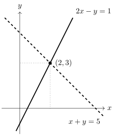
The row picture. Each equation describes a line in the plane: $y = 2x - 1$ and $y = 5 - x$ . A solution is a point on both lines, so solving the system means intersecting them. The lines meet at $(2, 3)$ .

Diagram. Labels: x, y, 2x - y = 1, x + y = 5, (2, 3)

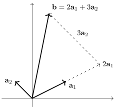
The column picture. Stack the coefficients of $x$ into one column and those of $y$ into another. The system says $x \begin{pmatrix} 2 \\ 1 \end{pmatrix} + y \begin{pmatrix} -1 \\ 1 \end{pmatrix} = \begin{pmatrix} 1 \\ 5 \end{pmatrix} .$ Now the unknowns are weights. We are asked how much of the vector $\mathbf{a}_1 = (2, 1)$ and how much of $\mathbf{a}_2 = (-1, 1)$ to combine to reach $\mathbf{b} = (1, 5)$ . The answer $x = 2$ , $y = 3$ says: walk twice along $\mathbf{a}_1$ , then three times along $\mathbf{a}_2$ .

Diagram. Labels: mathbf a_1, mathbf a_2, 2mathbf a_1, 3mathbf a_2, mathbf b = 2mathbf a_1 + 3mathbf a_2

The matrix picture. Collect the coefficients into a matrix and the unknowns into a column. By the definition of matrix multiplication (Definition 0.9.9), the system is the single equation $\begin{pmatrix} 2 & -1 \\ 1 & 1 \end{pmatrix} \begin{pmatrix} x \\ y \end{pmatrix} = \begin{pmatrix} 1 \\ 5 \end{pmatrix}, \qquad \text{that is,} \qquad \mathbf{A}\mathbf{x} = \mathbf{b} .$

The three pictures say the same thing, and they are tied together by one fact from Chapter 0: $\mathbf{A}\mathbf{x} = x_1\mathbf{a}_1 + \dots + x_n\mathbf{a}_n$ , a combination of the columns of $\mathbf{A}$ weighted by the entries of $\mathbf{x}$ (Theorem 0.9.3). The row picture is the one we draw. The column picture connects to Chapter 1, since it asks whether $\mathbf{b}$ lies in a span. The matrix picture is the one we compute and prove things with.

Remark. With more unknowns the pictures can no longer be drawn, but they do not change. An equation in three unknowns whose coefficients are not all zero describes a plane in $\mathbb{R}^3$ , and a system asks where several planes meet. In the column picture, three unknowns mean three columns, and we ask whether a combination of them hits $\mathbf{b}$ .

3.1.2. Linear systems

The example had two equations and two unknowns over $\mathbb{R}$ . The general notion allows any numbers of each, and any field. Allowing any field is not generality for its own sake. Systems over $\mathbb{F}_2$ describe parity checks and switching puzzles, and systems over $\mathbb{Q}$ are what a computer can solve exactly.

A linear system is a finite list of equations, each saying that a fixed combination of the unknowns equals a fixed scalar.

Definition 3.1.1 (Linear system)

Let $F$ be a field and let $m, n \ge 1$ . A system of $m$ linear equations in $n$ unknowns $x_1, \dots, x_n$ over $F$ is a list of equations $\begin{aligned} a_{11}x_1 + a_{12}x_2 + \dots + a_{1n}x_n &= b_1, \\ a_{21}x_1 + a_{22}x_2 + \dots + a_{2n}x_n &= b_2, \\ &\ \ \vdots \\ a_{m1}x_1 + a_{m2}x_2 + \dots + a_{mn}x_n &= b_m, \end{aligned}$ where all $a_{ij}$ and $b_i$ lie in $F$ .

The coefficient matrix is $\mathbf{A} = (a_{ij}) \in M_{m \times n}(F)$ , the right-hand side is $\mathbf{b} = (b_1, \dots, b_m) \in F^m$ , and the system is written $\mathbf{A}\mathbf{x} = \mathbf{b}$ .
The augmented matrix is the $m \times (n + 1)$ matrix $[\, \mathbf{A} \mid \mathbf{b} \,]$ obtained by appending $\mathbf{b}$ to $\mathbf{A}$ as a last column.
A solution is a vector $\mathbf{s} = (s_1, \dots, s_n) \in F^n$ such that every equation holds when $x_j = s_j$ for all $j$ ; equivalently, $\mathbf{A}\mathbf{s} = \mathbf{b}$ . The solution set is the set of all solutions, a subset of $F^n$ .
The system is consistent if it has at least one solution, and inconsistent if its solution set is empty.

In words: the coefficient matrix records the left-hand sides, row $i$ for equation $i$ and column $j$ for unknown $x_j$ . The augmented matrix records the whole system, and it is the object we will manipulate in the next section. A solution is a single vector of $F^n$ , and it must satisfy all $m$ equations at once, not just some of them. “Equivalently, $\mathbf{A}\mathbf{s} = \mathbf{b}$ ” holds because the $i$ -th entry of $\mathbf{A}\mathbf{s}$ is $a_{i1}s_1 + \dots + a_{in}s_n$ by Definition 0.9.9, and two columns are equal exactly when all their entries agree.

Two small words deserve attention. A solution lives in $F^n$ , with entries in the field $F$ : the equation $2x = 1$ has the solution $\tfrac12$ over $\mathbb{Q}$ , but over $\mathbb{F}_2$ it reads $0 = 1$ and has none. And “consistent” means at least one solution, not exactly one.

Example (None, one, or a whole line)

Find the solution set of each system over $\mathbb{R}$ , and describe it in the row picture.

(a) $x + 2y = 1$ , $2x + 4y = 5$ .
(b) $2x - y = 1$ , $x + y = 5$ .
(c) $x + 2y = 1$ , $2x + 4y = 2$ .

Solution.

(a) Suppose $(x, y)$ is a solution. Doubling the first equation gives $2x + 4y = 2$ , while the second says $2x + 4y = 5$ . Then $2 = 5$ , which is false. So there is no solution, and the system is inconsistent. In the row picture, the lines $y = \tfrac12 - \tfrac12 x$ and $y = \tfrac54 - \tfrac12 x$ have the same slope and different intercepts: they are parallel and never meet.
(b) As computed at the start of the section, any solution has $x = 2$ and $y = 3$ ; conversely $2 \cdot 2 - 3 = 1$ and $2 + 3 = 5$ . The solution set is $\{ (2, 3) \}$ , the single point where two non-parallel lines cross.
(c) The second equation is twice the first, so a pair $(x, y)$ satisfies both exactly when it satisfies $x + 2y = 1$ , that is, when $x = 1 - 2y$ . Writing $t$ for $y$ , the solution set is $\{ (1 - 2t, t) : t \in \mathbb{R} \}$ . Both equations describe the same line, and every point on it is a solution.

The three answers are the three things two lines can do: miss, cross, or coincide. Over $\mathbb{R}$ , and over any infinite field, no other sizes are possible: once we know the shape of the solution set (Theorem 3.1.3 below), this is a short argument, which you will give in Exercise (C1: How many solutions?). For instance, no system over $\mathbb{R}$ has exactly two solutions. Over a finite field the picture is different.

Example (Exactly two solutions over

\mathbb{F}_2

)

Find all solutions of the system $x + y + z = 1$ , $y + z = 0$ over $\mathbb{F}_2$ . Then compare with the same system over $\mathbb{R}$ .

Solution. In $\mathbb{F}_2$ we have $-1 = 1$ , so the second equation says $y = -z = z$ . Substituting into the first gives $x + 2z = 1$ , and $2z = 0$ in $\mathbb{F}_2$ , so $x = 1$ . Conversely, every $(1, z, z)$ satisfies both equations: $1 + z + z = 1 + 2z = 1$ and $z + z = 0$ . Since $z$ can only be $0$ or $1$ , the solution set is $\{ (1, 0, 0),\ (1, 1, 1) \},$ with exactly two elements.

Over $\mathbb{R}$ the second equation gives $y = -z$ , and then the first gives $x = 1$ . The solution set is $\{ (1, -t, t) : t \in \mathbb{R} \}$ , a line in $\mathbb{R}^3$ with infinitely many points. The equations are the same, but the field decides how many values the free unknown can take.

Now a non-example, by a minimal change. The equation $x + y^2 = 1$ looks like one of the equations above, and it still has a left side built from the unknowns and a constant on the right. But the unknown $y$ appears squared, so the left side is not of the form $a_1x_1 + a_2x_2$ with fixed scalars $a_1, a_2$ . The clause that fails is “a fixed combination of the unknowns”. Its solution set in $\mathbb{R}^2$ is a parabola, not a line, and nothing in this chapter applies to it.

Warning. “Consistent” does not mean “has exactly one solution”. The system $x + 2y = 1$ , $2x + 4y = 2$ of Example (None, one, or a whole line) (c) is consistent, and it has infinitely many solutions. Consistency only rules out the empty solution set. Whether the solution is unique is a separate question, answered by Corollary 3.1.4 below.

Why record the augmented matrix at all, when $\mathbf{A}\mathbf{x} = \mathbf{b}$ is shorter? Because solving a system never touches the names of the unknowns. Adding two equations adds their coefficients and their right-hand sides, and nothing else. The augmented matrix keeps exactly this data and throws away the symbols $x_1, \dots, x_n$ and the plus signs. In the next section every manipulation is performed on it.

One kind of system is always consistent, because it has an obvious solution.

Definition 3.1.2 (Homogeneous system)

A linear system $\mathbf{A}\mathbf{x} = \mathbf{b}$ over $F$ is homogeneous if $\mathbf{b} = \mathbf{0}$ . The vector $\mathbf{0} \in F^n$ is a solution of every homogeneous system $\mathbf{A}\mathbf{x} = \mathbf{0}$ , called the trivial solution. For any system $\mathbf{A}\mathbf{x} = \mathbf{b}$ , the system $\mathbf{A}\mathbf{x} = \mathbf{0}$ , with the same coefficient matrix, is its associated homogeneous system.

The trivial solution exists by the zero rule of Theorem 0.9.4: $\mathbf{A}\mathbf{0} = \mathbf{0}$ . So for a homogeneous system the interesting question is never “is there a solution?” but “is there a non-trivial one?”. For example, $x + 2y = 0$ , $2x + 4y = 0$ has the non-trivial solution $(-2, 1)$ , while $2x - y = 0$ , $x + y = 0$ has only the trivial one: adding the equations gives $3x = 0$ , so $x = 0$ , and then $y = -x = 0$ .

Quick check. Over $\mathbb{R}$ , write the system $x_1 - x_2 + 3x_3 = 4$ , $2x_2 + x_3 = 0$ in the matrix picture and the column picture, and give its augmented matrix. Is $(4, 0, 0)$ a solution? Is $(1, 0, 1)$ ?

Solution. With $\mathbf{A} = \begin{pmatrix} 1 & -1 & 3 \\ 0 & 2 & 1 \end{pmatrix}$ and $\mathbf{b} = (4, 0)$ , the system is $\mathbf{A}\mathbf{x} = \mathbf{b}$ . In the column picture it reads $x_1(1, 0) + x_2(-1, 2) + x_3(3, 1) = (4, 0)$ . The augmented matrix is $[\, \mathbf{A} \mid \mathbf{b} \,] = \left[ \begin{array}{ccc|c} 1 & -1 & 3 & 4 \\ 0 & 2 & 1 & 0 \end{array} \right].$ For $(4, 0, 0)$ : $4 - 0 + 0 = 4$ and $0 + 0 = 0$ , so it is a solution. For $(1, 0, 1)$ : the first equation gives $1 - 0 + 3 = 4$ , but the second gives $0 + 1 = 1 \neq 0$ . One failing equation is enough, so it is not a solution.

3.1.3. Consistency is a question about span

The column picture turns “does this system have a solution?” into a question from Chapter 1.

Theorem 3.1.1 (Consistency and the span of the columns)

Let $\mathbf{A} \in M_{m \times n}(F)$ have columns $\mathbf{a}_1, \dots, \mathbf{a}_n \in F^m$ , and let $\mathbf{b} \in F^m$ . Then the system $\mathbf{A}\mathbf{x} = \mathbf{b}$ is consistent if and only if $\mathbf{b} \in \operatorname{span}(\mathbf{a}_1, \dots, \mathbf{a}_n)$ . More precisely, $\mathbf{s} = (s_1, \dots, s_n)$ is a solution exactly when $\mathbf{b} = s_1\mathbf{a}_1 + \dots + s_n\mathbf{a}_n$ .

Proof. By Theorem 0.9.3, $\mathbf{A}\mathbf{s} = s_1\mathbf{a}_1 + \dots + s_n\mathbf{a}_n$ for every $\mathbf{s} \in F^n$ . Hence $\mathbf{s}$ is a solution, that is $\mathbf{A}\mathbf{s} = \mathbf{b}$ , exactly when $\mathbf{b} = s_1\mathbf{a}_1 + \dots + s_n\mathbf{a}_n$ . This proves the second statement.

$(\Rightarrow)$ If the system is consistent, it has a solution $\mathbf{s}$ , and then $\mathbf{b} = s_1\mathbf{a}_1 + \dots + s_n\mathbf{a}_n$ is a linear combination of the columns. By Definition 1.3.2, $\mathbf{b} \in \operatorname{span}(\mathbf{a}_1, \dots, \mathbf{a}_n)$ .

$(\Leftarrow)$ If $\mathbf{b} \in \operatorname{span}(\mathbf{a}_1, \dots, \mathbf{a}_n)$ , then $\mathbf{b} = s_1\mathbf{a}_1 + \dots + s_n\mathbf{a}_n$ for some $s_1, \dots, s_n \in F$ , and $\mathbf{s} = (s_1, \dots, s_n)$ is a solution by the first paragraph. Hence the system is consistent.

Read backwards, the theorem is a recipe for Chapter 1 questions: to decide whether $\mathbf{b}$ lies in the span of some vectors of $F^m$ , put the vectors as the columns of a matrix and ask whether the system is consistent.

Example (Span membership as a system)

In $\mathbb{R}^3$ , let $\mathbf{v}_1 = (1, 2, 3)$ and $\mathbf{v}_2 = (0, 1, 2)$ . Decide whether $(1, 4, 7)$ and $(1, 4, 8)$ lie in $\operatorname{span}(\mathbf{v}_1, \mathbf{v}_2)$ .

Solution. Let $\mathbf{A}$ be the $3 \times 2$ matrix with columns $\mathbf{v}_1, \mathbf{v}_2$ . By Theorem 3.1.1, $(1, 4, 7) \in \operatorname{span}(\mathbf{v}_1, \mathbf{v}_2)$ if and only if the system $a = 1, \qquad 2a + b = 4, \qquad 3a + 2b = 7$ in the unknowns $a, b$ is consistent. The first equation gives $a = 1$ , and then the second gives $b = 2$ . The third equation must also hold, and it does: $3 + 4 = 7$ . Hence $(1, 4, 7) = \mathbf{v}_1 + 2\mathbf{v}_2$ lies in the span.

For $(1, 4, 8)$ , the first two equations are the same, so any solution has $a = 1$ and $b = 2$ . The third equation now demands $3 + 4 = 8$ , which is false. The system is inconsistent, so $(1, 4, 8) \notin \operatorname{span}(\mathbf{v}_1, \mathbf{v}_2)$ .

Geometrically, $\operatorname{span}(\mathbf{v}_1, \mathbf{v}_2)$ is a plane through $\mathbf{0}$ in $\mathbb{R}^3$ . The first right-hand side lies on that plane and the second does not.

3.1.4. The shape of the solution set

We now describe the solution set of an arbitrary system, starting with the homogeneous case. Chapter 1 already did the work there: in Example (Solutions of a Homogeneous System) we checked, with the three conditions of the subspace test, that the solutions of $\mathbf{A}\mathbf{x} = \mathbf{0}$ form a subspace.

Theorem 3.1.2 (Homogeneous solutions form a subspace)

Let $\mathbf{A} \in M_{m \times n}(F)$ . The solution set $N = \{ \mathbf{x} \in F^n : \mathbf{A}\mathbf{x} = \mathbf{0} \}$ of the homogeneous system $\mathbf{A}\mathbf{x} = \mathbf{0}$ is a subspace of $F^n$ .

Proof. This is Example (Solutions of a Homogeneous System): $\mathbf{A}\mathbf{0} = \mathbf{0}$ , and for $\mathbf{x}, \mathbf{y} \in N$ and $c \in F$ , the rules of Theorem 0.9.4 give $\mathbf{A}(\mathbf{x} + \mathbf{y}) = \mathbf{A}\mathbf{x} + \mathbf{A}\mathbf{y} = \mathbf{0}$ and $\mathbf{A}(c\mathbf{x}) = c(\mathbf{A}\mathbf{x}) = \mathbf{0}$ . By the subspace test (Theorem 1.2.1), $N$ is a subspace of $F^n$ .

The solutions of $\mathbf{A}\mathbf{x} = \mathbf{b}$ with $\mathbf{b} \neq \mathbf{0}$ behave differently.

Warning. The solution set of $\mathbf{A}\mathbf{x} = \mathbf{b}$ with $\mathbf{b} \neq \mathbf{0}$ is never a subspace. A subspace must contain $\mathbf{0}$ , but $\mathbf{A}\mathbf{0} = \mathbf{0} \neq \mathbf{b}$ , so $\mathbf{0}$ is not a solution. For example, the solutions of $x - y = 1$ in $\mathbb{R}^2$ form a line that misses the origin. The sum of the solutions $(1, 0)$ and $(2, 1)$ is $(3, 1)$ , and $3 - 1 = 2 \neq 1$ : adding two solutions does not give a solution.

What does survive is this: the difference of two solutions of $\mathbf{A}\mathbf{x} = \mathbf{b}$ solves the homogeneous system, since $\mathbf{A}(\mathbf{s} - \mathbf{s}') = \mathbf{b} - \mathbf{b} = \mathbf{0}$ . So once one solution is known, every other one differs from it by a homogeneous solution. That is the whole structure.

Theorem 3.1.3 (Structure of the solution set)

Let $\mathbf{A} \in M_{m \times n}(F)$ and $\mathbf{b} \in F^m$ , let $N$ be the solution set of $\mathbf{A}\mathbf{x} = \mathbf{0}$ , and suppose $\mathbf{p} \in F^n$ is one solution of $\mathbf{A}\mathbf{x} = \mathbf{b}$ . Then the solution set of $\mathbf{A}\mathbf{x} = \mathbf{b}$ is $\mathbf{p} + N = \{ \mathbf{p} + \mathbf{h} : \mathbf{h} \in N \}.$

Idea. The theorem is “particular plus homogeneous”. To prove equality of two sets, prove both inclusions. Going from a solution $\mathbf{s}$ to $\mathbf{p} + N$ uses the difference $\mathbf{s} - \mathbf{p}$ , as observed above; going back uses the sum $\mathbf{A}(\mathbf{p} + \mathbf{h}) = \mathbf{A}\mathbf{p} + \mathbf{A}\mathbf{h}$ .

Proof. Let $S$ be the solution set of $\mathbf{A}\mathbf{x} = \mathbf{b}$ . We use Theorem 0.3.1.

$(\subseteq)$ Let $\mathbf{s} \in S$ , and put $\mathbf{h} = \mathbf{s} - \mathbf{p}$ . By distributivity (Theorem 0.9.4), $\mathbf{A}\mathbf{h} = \mathbf{A}\mathbf{s} - \mathbf{A}\mathbf{p} = \mathbf{b} - \mathbf{b} = \mathbf{0}$ , so $\mathbf{h} \in N$ . Hence $\mathbf{s} = \mathbf{p} + \mathbf{h} \in \mathbf{p} + N$ .

$(\supseteq)$ Let $\mathbf{h} \in N$ . Then $\mathbf{A}(\mathbf{p} + \mathbf{h}) = \mathbf{A}\mathbf{p} + \mathbf{A}\mathbf{h} = \mathbf{b} + \mathbf{0} = \mathbf{b}$ , again by distributivity, so $\mathbf{p} + \mathbf{h} \in S$ .

Therefore $S = \mathbf{p} + N$ , as claimed.

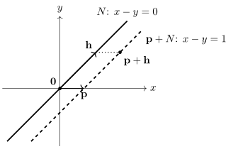
The theorem splits solving $\mathbf{A}\mathbf{x} = \mathbf{b}$ into two independent jobs: find one solution, and find all solutions of the homogeneous system. The set $\mathbf{p} + N$ is a translate of the subspace $N$ by the vector $\mathbf{p}$ , the kind of set that the picture in Example (A Line Missing the Origin) showed. For $x - y = 1$ in $\mathbb{R}^2$ , the homogeneous solutions form the line $N = \operatorname{span}((1, 1))$ through $\mathbf{0}$ , one solution is $\mathbf{p} = (1, 0)$ , and the solution set is the parallel line through $\mathbf{p}$ .

Diagram. Labels: x, y, N: x - y = 0, mathbf p + N: x - y = 1, mathbf 0, mathbf p, mathbf h, mathbf p + mathbf h

A system solved by substitution fits the same pattern once we collect the free parameter.

Example (Particular plus homogeneous)

Solve $x_1 + 2x_2 - x_3 = 4$ , $x_2 + x_3 = 1$ over $\mathbb{R}$ , and write the solution set in the form $\mathbf{p} + \operatorname{span}(\mathbf{h})$ .

Solution. The second equation gives $x_2 = 1 - x_3$ . Substituting into the first, $x_1 = 4 - 2(1 - x_3) + x_3 = 2 + 3x_3$ . The value of $x_3$ is not constrained, so write $x_3 = t$ . Conversely, for every $t \in \mathbb{R}$ the vector $(2 + 3t, 1 - t, t)$ satisfies both equations, since $(2 + 3t) + 2(1 - t) - t = 4$ and $(1 - t) + t = 1$ . Hence the solution set is $\{ (2 + 3t, 1 - t, t) : t \in \mathbb{R} \} = \{ (2, 1, 0) + t(3, -1, 1) : t \in \mathbb{R} \} = \mathbf{p} + \operatorname{span}(\mathbf{h}),$ with $\mathbf{p} = (2, 1, 0)$ and $\mathbf{h} = (3, -1, 1)$ . As Theorem 3.1.3 predicts, $\mathbf{p}$ is a solution (take $t = 0$ ), and $\mathbf{h}$ solves the homogeneous system: $3 - 2 - 1 = 0$ and $-1 + 1 = 0$ . In the row picture, two planes in $\mathbb{R}^3$ meet in a line, and this line does not pass through $\mathbf{0}$ .

3.1.5. When is the solution unique?

A consistent system has a unique solution exactly when there is nothing to add to the particular solution. The theorem just proved turns this into a statement about the homogeneous system, and the column picture turns that into independence.

Corollary 3.1.4 (Uniqueness of solutions)

Let $\mathbf{A} \in M_{m \times n}(F)$ have columns $\mathbf{a}_1, \dots, \mathbf{a}_n$ , and let $\mathbf{b} \in F^m$ be such that $\mathbf{A}\mathbf{x} = \mathbf{b}$ is consistent. The following are equivalent:

(a) $\mathbf{A}\mathbf{x} = \mathbf{b}$ has exactly one solution;
(b) $\mathbf{A}\mathbf{x} = \mathbf{0}$ has only the trivial solution;
(c) the list $(\mathbf{a}_1, \dots, \mathbf{a}_n)$ is linearly independent.

Proof. Let $N$ be the solution set of $\mathbf{A}\mathbf{x} = \mathbf{0}$ . Since the system is consistent, it has a solution $\mathbf{p}$ , and by Theorem 3.1.3 its solution set is $\mathbf{p} + N$ .

(a $\Leftrightarrow$ b) The function $N \to \mathbf{p} + N$ , $\mathbf{h} \mapsto \mathbf{p} + \mathbf{h}$ , is surjective by definition of $\mathbf{p} + N$ , and injective because $\mathbf{p} + \mathbf{h} = \mathbf{p} + \mathbf{h}'$ implies $\mathbf{h} = \mathbf{h}'$ by adding $-\mathbf{p}$ to both sides. So it is a bijection, and $\mathbf{p} + N$ has exactly one element if and only if $N$ does. Since $\mathbf{0} \in N$ always, $N$ has exactly one element if and only if $N = \{ \mathbf{0} \}$ , which is (b).

(b $\Leftrightarrow$ c) By Theorem 0.9.3, $\mathbf{A}\mathbf{x} = x_1\mathbf{a}_1 + \dots + x_n\mathbf{a}_n$ for every $\mathbf{x} \in F^n$ . So (b) says: for all $x_1, \dots, x_n \in F$ , $x_1\mathbf{a}_1 + \dots + x_n\mathbf{a}_n = \mathbf{0}$ implies $x_1 = \dots = x_n = 0$ . This is word for word Definition 1.4.1 for the list $(\mathbf{a}_1, \dots, \mathbf{a}_n)$ .

Two remarks on the hypotheses. The equivalence of (b) and (c) does not need consistency; only (a) does. And consistency cannot be dropped from (a $\Leftrightarrow$ b): the system $x = 0$ , $x = 1$ in one unknown has only the trivial solution in its homogeneous version ( $x = 0$ , $x = 0$ ), but it has no solution at all, so it certainly does not have exactly one.

So the three pictures answer the two basic questions about $\mathbf{A}\mathbf{x} = \mathbf{b}$ in the language of Chapter 1: a solution exists when $\mathbf{b}$ is in the span of the columns, and it is unique when the columns are independent. What we still lack is a reliable way to decide either question for a given matrix. That is the job of Gaussian elimination, in the next section.

3.1.6. Exercises

A. Check your understanding

Exercise (A1)

(a) Define what it means for a linear system $\mathbf{A}\mathbf{x} = \mathbf{b}$ over $F$ to be consistent, and what its augmented matrix is. What is the size of the augmented matrix of a system of $m$ equations in $n$ unknowns?
(b) Determine whether the following statement is true: “the solution set of $\mathbf{A}\mathbf{x} = \mathbf{b}$ is a subspace of $F^n$ .” Justify your answer.
(c) Determine whether the following statement is true: “if $\mathbf{A}\mathbf{x} = \mathbf{b}$ has two different solutions, then $\mathbf{A}\mathbf{x} = \mathbf{0}$ has a non-trivial solution.” Justify your answer.
(d) Let $\mathbf{A} \in M_{3 \times 5}(\mathbb{R})$ . In which spaces do the unknown vector $\mathbf{x}$ and the right-hand side $\mathbf{b}$ of $\mathbf{A}\mathbf{x} = \mathbf{b}$ live?
(e) Name the theorem that turns “is $\mathbf{b}$ in the span of $\mathbf{a}_1, \dots, \mathbf{a}_n$ ?” into a question about a linear system, and state which system.

Solution.

(a) It is consistent if it has at least one solution $\mathbf{s} \in F^n$ , that is, some $\mathbf{s}$ with $\mathbf{A}\mathbf{s} = \mathbf{b}$ . The augmented matrix is $[\, \mathbf{A} \mid \mathbf{b} \,]$ , the matrix $\mathbf{A}$ with $\mathbf{b}$ appended as an extra last column. It has size $m \times (n + 1)$ .
(b) False in general. If $\mathbf{b} \neq \mathbf{0}$ , then $\mathbf{A}\mathbf{0} = \mathbf{0} \neq \mathbf{b}$ , so $\mathbf{0}$ is not a solution and the solution set is not a subspace. (If $\mathbf{b} = \mathbf{0}$ , it is a subspace, by Theorem 3.1.2.)
(c) True. If $\mathbf{s} \neq \mathbf{s}'$ are solutions, then $\mathbf{A}(\mathbf{s} - \mathbf{s}') = \mathbf{b} - \mathbf{b} = \mathbf{0}$ by distributivity, and $\mathbf{s} - \mathbf{s}' \neq \mathbf{0}$ .
(d) $\mathbf{x} \in \mathbb{R}^5$ , one entry per column of $\mathbf{A}$ , and $\mathbf{b} \in \mathbb{R}^3$ , one entry per row.
(e) Theorem 3.1.1: $\mathbf{b} \in \operatorname{span}(\mathbf{a}_1, \dots, \mathbf{a}_n)$ if and only if $\mathbf{A}\mathbf{x} = \mathbf{b}$ is consistent, where $\mathbf{A}$ is the matrix with columns $\mathbf{a}_1, \dots, \mathbf{a}_n$ .

B. Practice

Exercise (B1: Three views)

(a) Write the system $x_1 - x_2 + 2x_3 = 3$ , $2x_1 + x_3 = 1$ over $\mathbb{R}$ in the matrix picture and in the column picture, and give its augmented matrix.
(b) Write out, as a list of equations, the system with augmented matrix $\left[ \begin{array}{cc|c} 1 & 4 & 0 \\ 0 & 1 & 2 \\ 3 & -1 & 5 \end{array} \right]$ over $\mathbb{R}$ . How many equations and unknowns does it have? Hence decide whether it is consistent.

Solution.

(a) The matrix picture is $\begin{pmatrix} 1 & -1 & 2 \\ 2 & 0 & 1 \end{pmatrix} \begin{pmatrix} x_1 \\ x_2 \\ x_3 \end{pmatrix} = \begin{pmatrix} 3 \\ 1 \end{pmatrix}.$ The column picture is $x_1(1, 2) + x_2(-1, 0) + x_3(2, 1) = (3, 1)$ . The augmented matrix is $\left[ \begin{array}{ccc|c} 1 & -1 & 2 & 3 \\ 2 & 0 & 1 & 1 \end{array} \right]$ .
(b) The system is $x_1 + 4x_2 = 0$ , $x_2 = 2$ , $3x_1 - x_2 = 5$ : three equations in two unknowns. The second equation gives $x_2 = 2$ , and then the first gives $x_1 = -8$ . The third equation would require $-24 - 2 = 5$ , which is false. Hence no vector satisfies all three equations, and the system is inconsistent.

Exercise (B2: In the span or not?)

Determine whether the vector $\mathbf{b}$ lies in the span of the given vectors. Justify your answer, and when it does, write $\mathbf{b}$ as a linear combination of them.

(a) $\mathbf{b} = (2, 1, 4)$ and $(1, 0, 1), (0, 1, 2)$ in $\mathbb{R}^3$ .
(b) $\mathbf{b} = (1, 1, 1)$ and $(1, 2, 0), (2, 4, 1)$ in $\mathbb{R}^3$ .
(c) $\mathbf{b} = (1, 1, 0)$ and $(1, 0, 1), (0, 1, 1)$ in $\mathbb{F}_2^3$ . Is the answer the same in $\mathbb{R}^3$ ?

Solution. By Theorem 3.1.1, in each case we decide whether the system $a\mathbf{v}_1 + b\mathbf{v}_2 = \mathbf{b}$ in the unknowns $a, b$ is consistent.

(a) The system is $a = 2$ , $b = 1$ , $a + 2b = 4$ . The first two equations force $a = 2$ , $b = 1$ , and then $a + 2b = 4$ holds. Hence $(2, 1, 4) = 2(1, 0, 1) + (0, 1, 2)$ is in the span.
(b) The system is $a + 2b = 1$ , $2a + 4b = 1$ , $b = 1$ . Doubling the first equation gives $2a + 4b = 2$ , contradicting the second, since $2 \neq 1$ . Hence the system is inconsistent and $(1, 1, 1)$ is not in the span.
(c) The system is $a = 1$ , $b = 1$ , $a + b = 0$ . The first two force $a = b = 1$ , and then $a + b = 1 + 1 = 0$ in $\mathbb{F}_2$ . Hence $(1, 1, 0) = (1, 0, 1) + (0, 1, 1)$ is in the span over $\mathbb{F}_2$ . In $\mathbb{R}^3$ the same first two equations force $a = b = 1$ , but $1 + 1 = 2 \neq 0$ , so the system is inconsistent and $\mathbf{b}$ is not in the span. The answer depends on the field.

Exercise (B3: Solve and describe)

Solve each system over $\mathbb{R}$ by substitution, and write its solution set in the form $\mathbf{p} + \operatorname{span}(\dots)$ . Check that your $\mathbf{p}$ is a solution and that your spanning vectors solve the associated homogeneous system.

(a) $x_1 + x_2 + x_3 = 2$ , $x_2 - x_3 = 1$ .
(b) $x_1 - 2x_2 + x_3 - x_4 = 1$ , $x_3 + 2x_4 = 3$ .

Solution.

(a) The second equation gives $x_2 = 1 + x_3$ , and then the first gives $x_1 = 2 - (1 + x_3) - x_3 = 1 - 2x_3$ . With $x_3 = t$ free, every solution is $(1 - 2t, 1 + t, t)$ , and conversely each such vector satisfies both equations. So the solution set is $(1, 1, 0) + \operatorname{span}((-2, 1, 1))$ . Check: $1 + 1 + 0 = 2$ and $1 - 0 = 1$ ; and $-2 + 1 + 1 = 0$ , $1 - 1 = 0$ .
(b) The second equation gives $x_3 = 3 - 2x_4$ . The first then gives $x_1 = 1 + 2x_2 - (3 - 2x_4) + x_4 = -2 + 2x_2 + 3x_4$ . The unknowns $x_2 = s$ and $x_4 = t$ are free, and every solution is $(-2 + 2s + 3t,\ s,\ 3 - 2t,\ t) = (-2, 0, 3, 0) + s(2, 1, 0, 0) + t(3, 0, -2, 1),$ and conversely each such vector is a solution. So the solution set is $(-2, 0, 3, 0) + \operatorname{span}((2, 1, 0, 0), (3, 0, -2, 1))$ . Check: $-2 - 0 + 3 - 0 = 1$ and $3 + 0 = 3$ ; for $(2, 1, 0, 0)$ : $2 - 2 + 0 - 0 = 0$ and $0 + 0 = 0$ ; for $(3, 0, -2, 1)$ : $3 - 0 - 2 - 1 = 0$ and $-2 + 2 = 0$ .

C. Going deeper

Exercise (C1: How many solutions?)

Let $\mathbf{A} \in M_{m \times n}(F)$ and $\mathbf{b} \in F^m$ , and let $N$ be the solution set of $\mathbf{A}\mathbf{x} = \mathbf{0}$ .

(a) Suppose $F$ is infinite. Prove that $\mathbf{A}\mathbf{x} = \mathbf{b}$ has either no solution, exactly one solution, or infinitely many solutions.
(b) Suppose $F$ is finite. Prove that $\mathbf{A}\mathbf{x} = \mathbf{b}$ has either no solution or exactly $\lvert N \rvert$ solutions.
(c) Give a system over $\mathbb{F}_3$ with exactly three solutions.

Hint: for (a), if $N$ contains a non-zero vector $\mathbf{h}$ , look at its multiples.

Solution.

(a) Suppose the system is consistent, with a solution $\mathbf{p}$ . By Theorem 3.1.3 its solution set is $\mathbf{p} + N$ , and as in the proof of Corollary 3.1.4 the map $\mathbf{h} \mapsto \mathbf{p} + \mathbf{h}$ is a bijection $N \to \mathbf{p} + N$ . If $N = \{ \mathbf{0} \}$ , there is exactly one solution. Otherwise, let $\mathbf{h} \in N$ with $\mathbf{h} \neq \mathbf{0}$ . Since $N$ is a subspace (Theorem 3.1.2), $c\mathbf{h} \in N$ for every $c \in F$ . If $c\mathbf{h} = c'\mathbf{h}$ , then $(c - c')\mathbf{h} = \mathbf{0}$ , and since $\mathbf{h} \neq \mathbf{0}$ , Theorem 1.1.9 gives $c = c'$ . So $c \mapsto c\mathbf{h}$ is injective, and $N$ contains infinitely many vectors because $F$ is infinite. Hence $\mathbf{p} + N$ is infinite.
(b) If the system is consistent with solution $\mathbf{p}$ , the bijection $N \to \mathbf{p} + N$ from (a) shows that the solution set has exactly $\lvert N \rvert$ elements. Otherwise it has none.
(c) The single equation $x + y = 1$ over $\mathbb{F}_3$ (a system with $m = 1$ , $n = 2$ ). For each of the three values of $y \in \mathbb{F}_3$ there is exactly one $x = 1 - y$ , so the solutions are $(1, 0), (0, 1), (2, 2)$ . Consistently with (b), the homogeneous equation $x + y = 0$ has the three solutions $(0, 0), (2, 1), (1, 2)$ .

Exercise (C2: The right-hand sides that work)

Let $\mathbf{A} \in M_{m \times n}(F)$ have columns $\mathbf{a}_1, \dots, \mathbf{a}_n$ .

(a) Prove that the set $C = \{ \mathbf{b} \in F^m : \mathbf{A}\mathbf{x} = \mathbf{b} \text{ is consistent} \}$ is a subspace of $F^m$ .
(b) Deduce that if $n < m$ , then there is some $\mathbf{b} \in F^m$ for which $\mathbf{A}\mathbf{x} = \mathbf{b}$ is inconsistent.
(c) For $\mathbf{A} = \begin{pmatrix} 1 & 2 \\ 2 & 4 \\ 0 & 1 \end{pmatrix}$ over $\mathbb{R}$ , find one such $\mathbf{b}$ .

Solution.

(a) By Theorem 3.1.1, $\mathbf{b} \in C$ if and only if $\mathbf{b} \in \operatorname{span}(\mathbf{a}_1, \dots, \mathbf{a}_n)$ . So $C = \operatorname{span}(\mathbf{a}_1, \dots, \mathbf{a}_n)$ , which is a subspace of $F^m$ by Theorem 1.3.1.
(b) By (a), $C$ is spanned by the $n$ vectors $\mathbf{a}_1, \dots, \mathbf{a}_n$ . Since $\dim F^m = m$ (Example (Dimensions of the Running Examples)), Theorem 1.6.3 says no list of fewer than $m$ vectors spans $F^m$ . As $n < m$ , $C \neq F^m$ , so some $\mathbf{b} \in F^m$ is not in $C$ , and for that $\mathbf{b}$ the system is inconsistent.
(c) Take $\mathbf{b} = (1, 0, 0)$ . A solution would satisfy $x + 2y = 1$ and $2x + 4y = 0$ . Doubling the first gives $2x + 4y = 2 \neq 0$ , a contradiction. So $\mathbf{A}\mathbf{x} = (1, 0, 0)$ is inconsistent.