13.8 The Singular Value Decomposition

Chapter 12 answered one question completely: an operator has an orthonormal basis of eigenvectors exactly when it is normal. That answer is useless for a $3 \times 5$ matrix, which has no eigenvalues at all — the equation $\mathbf{A}\mathbf{x} = \lambda\mathbf{x}$ is not even type-correct, because $\mathbf{A}\mathbf{x}$ and $\mathbf{x}$ live in different spaces. This section shows that every matrix, of every shape, still admits an orthonormal-to-orthogonal description, and that the numbers in it are the eigenvalues of a positive semidefinite matrix we already understand. It is the most-used factorization in applied linear algebra, and the whole of it comes from applying the spectral theorem to $\mathbf{A}^{*}\mathbf{A}$ .

Throughout, $F$ is $\mathbb{R}$ or $\mathbb{C}$ , $\mathbf{A}^{*}$ is the conjugate transpose (the transpose when $F = \mathbb{R}$ ), and unitary means unitary over $\mathbb{C}$ and orthogonal over $\mathbb{R}$ , as in Definition 11.7.2. Both $F^m$ and $F^n$ carry their standard inner products.

13.8.1. Where to look when there are no eigenvalues

Let $\mathbf{A} \in M_{m \times n}(F)$ . There is exactly one square matrix that can be built from $\mathbf{A}$ at no cost, and Chapter 11 has already used it twice: the $n \times n$ matrix $\mathbf{A}^{*}\mathbf{A}$ of the normal equations. It is self-adjoint, since $(\mathbf{A}^{*}\mathbf{A})^{*} = \mathbf{A}^{*}\mathbf{A}^{**} = \mathbf{A}^{*}\mathbf{A}$ , and it is positive semidefinite for the reason that makes every argument in this chapter work:

\langle \mathbf{A}^{*}\mathbf{A}\mathbf{x}, \mathbf{x} \rangle = \langle \mathbf{A}\mathbf{x}, \mathbf{A}\mathbf{x} \rangle = \left\| \mathbf{A}\mathbf{x} \right\|^2 \ge 0 .

(13.8.1)

So $\mathbf{A}^{*}\mathbf{A} \succeq 0$ , and Theorem 13.1.4 says its eigenvalues are non-negative real numbers, while the spectral theorem supplies an orthonormal basis of $F^n$ consisting of its eigenvectors. Those eigenvalues are attached to $\mathbf{A}$ , they exist for every shape of $\mathbf{A}$ , and Eq. 13.8.1 says what they measure: how much $\mathbf{A}$ stretches.

A rectangular matrix has no eigenvalues of its own, but $\mathbf{A}^{*}\mathbf{A}$ does, and their square roots are the stretching factors of $\mathbf{A}$ .

Definition 13.8.1 (Singular Values)

Let $\mathbf{A} \in M_{m \times n}(F)$ and put $p = \min(m, n)$ . Let $\lambda_1 \ge \lambda_2 \ge \dots \ge \lambda_n \ge 0$ be the eigenvalues of $\mathbf{A}^{*}\mathbf{A} \in M_n(F)$ , listed with multiplicity in decreasing order. The singular values of $\mathbf{A}$ are $\sigma_i(\mathbf{A}) \mathrel{:=} \sqrt{\lambda_i} \qquad (i = 1, \dots, p),$ so that $\sigma_1(\mathbf{A}) \ge \sigma_2(\mathbf{A}) \ge \dots \ge \sigma_p(\mathbf{A}) \ge 0$ . We write $\sigma_i$ when $\mathbf{A}$ is clear.

Clause by clause. The list has exactly $p = \min(m, n)$ entries, not $n$ : when $n > m$ the matrix $\mathbf{A}^{*}\mathbf{A}$ has rank $\operatorname{rank} \mathbf{A} \le m < n$ by Corollary 11.6.6 (b), so $\lambda_{m+1} = \dots = \lambda_n = 0$ and the discarded eigenvalues are all zero. The square root is the ordinary non-negative real square root, available because every $\lambda_i \ge 0$ . The ordering is decreasing, matching the book’s convention $\lambda_1(\mathbf{A}) \ge \dots \ge \lambda_n(\mathbf{A})$ for the eigenvalues of a Hermitian matrix, and it is part of the definition: “the second singular value” means a definite number. Finally, the singular values are attached to $\mathbf{A}$ itself, with no choices made, because the eigenvalue list of $\mathbf{A}^{*}\mathbf{A}$ is.

Four examples, simplest first.

The identity. $\mathbf{A} = \mathbf{I}_n$ gives $\mathbf{A}^{*}\mathbf{A} = \mathbf{I}_n$ , so every $\sigma_i = 1$ . More generally a unitary $\mathbf{U} \in M_n(F)$ has $\mathbf{U}^{*}\mathbf{U} = \mathbf{I}$ , so all its singular values are $1$ . A unitary matrix stretches nothing in any direction, and the list of singular values says exactly that.
A rectangular diagonal matrix. If $\mathbf{A} \in M_{m \times n}(F)$ has $a_{ii} = d_i$ for $i \le p$ and all other entries $0$ , then $\mathbf{A}^{*}\mathbf{A} = \operatorname{diag}(\lvert d_1\rvert^2, \dots)$ and the singular values are $\lvert d_1 \rvert, \dots, \lvert d_p \rvert$ sorted downwards. The absolute value matters: the singular values of $\operatorname{diag}(1, -2)$ are $2, 1$ .
A positive semidefinite matrix. If $\mathbf{A} \succeq 0$ then $\mathbf{A}^{*}\mathbf{A} = \mathbf{A}^2$ , whose eigenvalues are $\lambda_i(\mathbf{A})^2$ with $\lambda_i(\mathbf{A}) \ge 0$ , so $\sigma_i(\mathbf{A}) = \lambda_i(\mathbf{A})$ . For the matrices this chapter started with, singular values and eigenvalues coincide.
A single row. For $\mathbf{A} = \mathbf{a}^{*} \in M_{1 \times n}(F)$ with $\mathbf{a} \ne \mathbf{0}$ , $p = 1$ and $\mathbf{A}^{*}\mathbf{A} = \mathbf{a}\mathbf{a}^{*}$ , whose non-zero eigenvalue is $\left\| \mathbf{a} \right\|^2$ . So $\sigma_1 = \left\| \mathbf{a} \right\|$ . The degenerate case $\mathbf{A} = \mathbf{0}$ has every $\sigma_i = 0$ , and it matters: it is the only matrix with $\sigma_1 = 0$ , since $\sigma_1 = 0$ forces $\mathbf{A}^{*}\mathbf{A} = \mathbf{0}$ and then $\left\| \mathbf{A}\mathbf{x} \right\|^2 = 0$ for every $\mathbf{x}$ by Eq. 13.8.1.

Now the non-example, by minimal change. Replace “square roots of the eigenvalues of $\mathbf{A}^{*}\mathbf{A}$ ” by “absolute values of the eigenvalues of $\mathbf{A}$ ”. For $\mathbf{A} \succeq 0$ , and more generally for any normal $\mathbf{A}$ , the two agree (Exercise (C3: Singular values equal to eigenvalue moduli)). But the second recipe is undefined for a non-square matrix, and for $\mathbf{N} = \begin{pmatrix} 0 & 1 \\ 0 & 0 \end{pmatrix}$ it returns $0, 0$ , while $\mathbf{N}^{*}\mathbf{N} = \operatorname{diag}(0, 1)$ gives the singular values $1, 0$ . The clause that fails is the one that does all the work: $\mathbf{A}^{*}\mathbf{A}$ is positive semidefinite for every $\mathbf{A}$ , whereas $\mathbf{A}$ itself may have no useful spectrum.

Warning. Singular values are not eigenvalues. The matrix $\mathbf{N}$ above has both eigenvalues equal to $0$ and largest singular value $1$ : it annihilates $\mathbf{e}_1$ but sends $\mathbf{e}_2$ to a unit vector, so calling it “small” because its spectrum is $\{0\}$ is wrong. Singular values are always real and non-negative; eigenvalues need not be either. The two lists agree, after taking absolute values, exactly for normal matrices — this is Exercise (C3: Singular values equal to eigenvalue moduli), and Chapter 12’s Schur inequality is what makes the converse true.

Quick check. What are the singular values of an orthogonal projection $\mathbf{P} \in M_n(F)$ onto an $r$ -dimensional subspace?

Solution. $\mathbf{P}^{*}\mathbf{P} = \mathbf{P}^2 = \mathbf{P}$ , because an orthogonal projection is self-adjoint and idempotent. So the eigenvalues of $\mathbf{P}^{*}\mathbf{P}$ are those of $\mathbf{P}$ , namely $1$ with multiplicity $r$ and $0$ with multiplicity $n - r$ . Sorted downwards, the singular values are $\sigma_1 = \dots = \sigma_r = 1$ and $\sigma_{r+1} = \dots = \sigma_n = 0$ . This is also Example 3 above, since $\mathbf{P} \succeq 0$ .

13.8.2. The theorem

Here is the payoff. The eigenvectors of $\mathbf{A}^{*}\mathbf{A}$ are an orthonormal basis of the domain; the claim is that $\mathbf{A}$ carries them to an orthogonal list in the codomain, whose lengths are the singular values.

Theorem 13.8.1 (Singular Value Decomposition)

Let $\mathbf{A} \in M_{m \times n}(F)$ , let $p = \min(m, n)$ and let $\sigma_1 \ge \dots \ge \sigma_p \ge 0$ be its singular values. Then there are unitary matrices $\mathbf{U} \in M_m(F)$ and $\mathbf{V} \in M_n(F)$ such that $\mathbf{A} = \mathbf{U}\boldsymbol{\Sigma}\mathbf{V}^{*} ,$ where $\boldsymbol{\Sigma} \in M_{m \times n}(\mathbb{R})$ has $(\boldsymbol{\Sigma})_{ii} = \sigma_i$ for $i = 1, \dots, p$ and every other entry $0$ . Moreover the number of non-zero $\sigma_i$ equals $\operatorname{rank} \mathbf{A}$ .

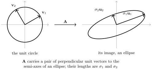
Idea. Picture the $2 \times 2$ real case. A matrix carries the unit circle to an ellipse, and an ellipse has two perpendicular axes; the theorem says that the two unit vectors sent to the ends of those axes are themselves perpendicular. That is exactly what Chapter 12’s principal axis theorem (Theorem 12.5.5) said about the level curves of a quadratic form, and the link is that $\left\| \mathbf{A}\mathbf{x} \right\|^2 = \mathbf{x}^{*}(\mathbf{A}^{*}\mathbf{A})\mathbf{x}$ is a quadratic form, with matrix $\mathbf{A}^{*}\mathbf{A}$ . So the plan is: ① diagonalize $\mathbf{A}^{*}\mathbf{A}$ by the spectral theorem, getting an orthonormal basis $\mathbf{v}_1, \dots, \mathbf{v}_n$ with $\mathbf{A}^{*}\mathbf{A}\mathbf{v}_i = \sigma_i^2\mathbf{v}_i$ ; ② compute $\langle \mathbf{A}\mathbf{v}_i, \mathbf{A}\mathbf{v}_j \rangle$ and watch the eigenvalue equation force it to be $\sigma_i^2\delta_{ij}$ , so the images are already orthogonal; ③ normalize the non-zero ones to unit vectors $\mathbf{u}_i$ , and, if there are fewer than $m$ of them, pad the list out to an orthonormal basis of $F^m$ ; ④ read $\mathbf{A}\mathbf{V} = \mathbf{U}\boldsymbol{\Sigma}$ off column by column.

Proof. Step 1: diagonalize $\mathbf{A}^{*}\mathbf{A}$ . The matrix $\mathbf{A}^{*}\mathbf{A} \in M_n(F)$ is self-adjoint, and Eq. 13.8.1 makes it positive semidefinite in the sense of Definition 13.1.1. By the spectral theorem in matrix form — Corollary 12.5.2 when $F = \mathbb{R}$ , Corollary 12.4.3 when $F = \mathbb{C}$ , each of which allows the eigenvalues to be listed in a prescribed order — there is a unitary $\mathbf{V} \in M_n(F)$ with columns $\mathbf{v}_1, \dots, \mathbf{v}_n$ such that $\mathbf{A}^{*}\mathbf{A}\,\mathbf{v}_i = \lambda_i\mathbf{v}_i, \qquad \lambda_1 \ge \dots \ge \lambda_n \ge 0 ,$ the eigenvalues being non-negative by Theorem 13.1.4. Set $\sigma_i = \sqrt{\lambda_i}$ for all $i \le n$ ; for $i \le p$ these are the singular values of Definition 13.8.1.

Step 2: the images are orthogonal. For all $i, j$ , using $\langle \mathbf{x}, \mathbf{y} \rangle = \mathbf{y}^{*}\mathbf{x}$ and the eigenvalue equation, $\langle \mathbf{A}\mathbf{v}_i, \mathbf{A}\mathbf{v}_j \rangle = \langle \mathbf{A}^{*}\mathbf{A}\mathbf{v}_i, \mathbf{v}_j \rangle = \lambda_i\langle \mathbf{v}_i, \mathbf{v}_j \rangle = \lambda_i\delta_{ij} ,$ the first equality by Definition 11.6.1 and the last because $\mathbf{V}$ is unitary, so its columns are orthonormal (Theorem 11.7.3 (f)). In particular $\left\| \mathbf{A}\mathbf{v}_i \right\|^2 = \lambda_i = \sigma_i^2$ , so

\mathbf{A}\mathbf{v}_i = \mathbf{0} \iff \sigma_i = 0 .

(13.8.2)

Step 3: normalize, and count. Let $r$ be the number of indices with $\sigma_i > 0$ ; since the $\sigma_i$ decrease, these are $i = 1, \dots, r$ . For $i \le r$ put $\mathbf{u}_i \mathrel{:=} \frac{1}{\sigma_i}\mathbf{A}\mathbf{v}_i ,$ which is legitimate because $\sigma_i \neq 0$ . By Step 2, $\langle \mathbf{u}_i, \mathbf{u}_j \rangle = \lambda_i\delta_{ij}/(\sigma_i\sigma_j) = \delta_{ij}$ for $i, j \le r$ , so $(\mathbf{u}_1, \dots, \mathbf{u}_r)$ is an orthonormal list in $F^m$ .

We claim $r = \operatorname{rank} \mathbf{A}$ . Any $\mathbf{x} \in F^n$ is $\mathbf{x} = \sum_i c_i\mathbf{v}_i$ since $(\mathbf{v}_1, \dots, \mathbf{v}_n)$ is a basis, and then $\mathbf{A}\mathbf{x} = \sum_{i \le r} c_i\sigma_i\mathbf{u}_i$ by Eq. 13.8.2. Hence $\operatorname{im} \mathbf{A} = \operatorname{span}(\mathbf{u}_1, \dots, \mathbf{u}_r)$ , and the $\mathbf{u}_i$ are orthonormal, hence independent (Theorem 11.1.4), so $\operatorname{rank} \mathbf{A} = r$ . In particular $r \le \min(m, n) = p$ , so every index $i$ with $\sigma_i > 0$ satisfies $i \le p$ , and the non-zero singular values are exactly $\sigma_1, \dots, \sigma_r$ .

Step 4: pad the list. If $r = m$ the list $(\mathbf{u}_1, \dots, \mathbf{u}_r)$ is already an orthonormal basis of $F^m$ , and we set $\mathbf{U} = (\mathbf{u}_1 \mid \dots \mid \mathbf{u}_m)$ . If $r < m$ , apply Corollary 11.2.3 to the orthonormal list $(\mathbf{u}_1, \dots, \mathbf{u}_r)$ in $F^m$ : there are $\mathbf{u}_{r+1}, \dots, \mathbf{u}_m$ making $(\mathbf{u}_1, \dots, \mathbf{u}_m)$ an orthonormal basis of $F^m$ . Either way let $\mathbf{U} \in M_m(F)$ have these columns; it is unitary because its columns are orthonormal (Theorem 11.7.3 (f)). Note that the padding vectors are not determined by $\mathbf{A}$ , and nothing below uses any property of them beyond orthonormality.

Step 5: read off the columns. Let $\boldsymbol{\Sigma} \in M_{m \times n}(\mathbb{R})$ be as in the statement. Column $i$ of $\mathbf{U}\boldsymbol{\Sigma}$ is $\mathbf{U}$ times column $i$ of $\boldsymbol{\Sigma}$ , which is $\sigma_i\mathbf{e}_i$ for $i \le p$ and $\mathbf{0}$ for $i > p$ ; so column $i$ of $\mathbf{U}\boldsymbol{\Sigma}$ is $\sigma_i\mathbf{u}_i$ for $i \le p$ and $\mathbf{0}$ for $i > p$ . Column $i$ of $\mathbf{A}\mathbf{V}$ is $\mathbf{A}\mathbf{v}_i$ . Compare:

for $i \le r$ , $\mathbf{A}\mathbf{v}_i = \sigma_i\mathbf{u}_i$ by the definition of $\mathbf{u}_i$ ;
for $r < i \le p$ , $\sigma_i = 0$ , so both columns are $\mathbf{0}$ by Eq. 13.8.2;
for $i > p$ (possible only when $n > m$ ), we have $i > p \ge r$ , so $\sigma_i = 0$ and $\mathbf{A}\mathbf{v}_i = \mathbf{0}$ , and both columns are $\mathbf{0}$ .

Hence $\mathbf{A}\mathbf{V} = \mathbf{U}\boldsymbol{\Sigma}$ . Since $\mathbf{V}$ is unitary, $\mathbf{V}^{-1} = \mathbf{V}^{*}$ , so $\mathbf{A} = \mathbf{U}\boldsymbol{\Sigma}\mathbf{V}^{*}$ . This proves the theorem.

A factorization $\mathbf{A} = \mathbf{U}\boldsymbol{\Sigma}\mathbf{V}^{*}$ as in the theorem is called a singular value decomposition of $\mathbf{A}$ , the columns $\mathbf{u}_i$ of $\mathbf{U}$ are left singular vectors and the columns $\mathbf{v}_i$ of $\mathbf{V}$ are right singular vectors. The two equations to keep in mind are the ones the proof produced,

\mathbf{A}\mathbf{v}_i = \sigma_i\mathbf{u}_i, \qquad \mathbf{A}^{*}\mathbf{u}_i = \sigma_i\mathbf{v}_i \qquad (i \le r),

(13.8.3)

the second obtained by applying $\mathbf{A}^{*}$ to the first and using $\mathbf{A}^{*}\mathbf{A}\mathbf{v}_i = \sigma_i^2\mathbf{v}_i$ . In words: $\mathbf{A}$ matches up two orthonormal bases, one in each space, stretching the $i$ -th direction by $\sigma_i$ , and $\mathbf{A}^{*}$ runs the same correspondence backwards with the same factors.

Remark. The last item on the invertibility list. For a square $\mathbf{A} \in M_n(F)$ , the count at the end of the theorem says that all $n$ singular values are non-zero exactly when $\operatorname{rank} \mathbf{A} = n$ , which is invertibility (Theorem 7.5.3 (d)). This is the item Chapter 3 promised when it began the list (Theorem 3.4.4), later grown in Theorem 7.5.3, Theorem 9.2.6 and Theorem 13.1.6, and it is the last one the book adds.

Here is the picture the Idea described, in the real $2 \times 2$ case.

$Diagram. Labels: A, v_1, v_2, the unit circle, sigma_1u_1, sigma_2u_2, its image, an ellipse, A carries a pair of perpendicular unit vectors to the\\ semi-axes of an ellipse; their lengths are sigma_1 and sigma_2$

Compare the principal axes figure of Chapter 12 §05. There the ellipse was a level curve $\mathbf{x}^{\top}\mathbf{A}\mathbf{x} = 1$ of a quadratic form and the axes lay along the eigenvectors of a symmetric $\mathbf{A}$ ; here the ellipse is the image of the unit circle under an arbitrary $\mathbf{A}$ . The two pictures are the same picture, because $\left\| \mathbf{A}\mathbf{x} \right\|^2 = \mathbf{x}^{*}(\mathbf{A}^{*}\mathbf{A})\mathbf{x}$ is a quadratic form with matrix $\mathbf{A}^{*}\mathbf{A}$ , and the right singular vectors of $\mathbf{A}$ are its principal axes. A large $\sigma_i$ now means a long semi-axis, whereas in Theorem 12.5.5 a large $\lambda_i$ meant a short one; the reason is that the two pictures are related by taking reciprocals of square roots.

13.8.3. What is unique and what is not

The singular values were defined before the theorem, so they cannot depend on any choice. What needs saying is the converse: any factorization of the stated shape recovers them.

Theorem 13.8.2 (The Singular Values Are Determined)

Let $\mathbf{A} \in M_{m \times n}(F)$ and suppose $\mathbf{A} = \mathbf{U}\boldsymbol{\Sigma}\mathbf{V}^{*}$ with $\mathbf{U}, \mathbf{V}$ unitary and $\boldsymbol{\Sigma} \in M_{m \times n}(\mathbb{R})$ of the shape in Theorem 13.8.1, with diagonal entries $s_1 \ge \dots \ge s_p \ge 0$ . Then $s_i = \sigma_i(\mathbf{A})$ for every $i$ . Moreover:

(a) the columns of $\mathbf{V}$ are forced to be an orthonormal basis of $F^n$ consisting of eigenvectors of $\mathbf{A}^{*}\mathbf{A}$ , with $\mathbf{A}^{*}\mathbf{A}\mathbf{v}_i = \sigma_i^2\mathbf{v}_i$ for every $i \le n$ , where $\sigma_i \mathrel{:=} 0$ for $p < i \le n$ ; and any such basis occurs;
(b) once $\mathbf{V}$ is chosen, $\mathbf{u}_i = \mathbf{A}\mathbf{v}_i/\sigma_i$ is forced for every $i \le r = \operatorname{rank}\mathbf{A}$ , while $\mathbf{u}_{r+1}, \dots, \mathbf{u}_m$ may be any orthonormal basis of $(\operatorname{im}\mathbf{A})^{\perp}$ .

Proof. From $\mathbf{A} = \mathbf{U}\boldsymbol{\Sigma}\mathbf{V}^{*}$ and $\mathbf{U}^{*}\mathbf{U} = \mathbf{I}_m$ , $\mathbf{A}^{*}\mathbf{A} = \mathbf{V}\boldsymbol{\Sigma}^{*}\mathbf{U}^{*}\mathbf{U}\boldsymbol{\Sigma}\mathbf{V}^{*} = \mathbf{V}(\boldsymbol{\Sigma}^{*}\boldsymbol{\Sigma})\mathbf{V}^{*} ,$ and $\boldsymbol{\Sigma}^{*}\boldsymbol{\Sigma} \in M_n(\mathbb{R})$ is the diagonal matrix with entries $s_1^2, \dots, s_p^2$ followed by zeros. So $\mathbf{A}^{*}\mathbf{A}$ is unitarily diagonalized with this diagonal, and its eigenvalue list in decreasing order is therefore $s_1^2 \ge \dots \ge s_p^2 \ge 0 \ge \dots$ — already sorted, since the $s_i$ are. Comparing with Definition 13.8.1 gives $s_i^2 = \sigma_i(\mathbf{A})^2$ , hence $s_i = \sigma_i(\mathbf{A})$ because both are non-negative.

(a) The displayed equation says the $i$ -th column of $\mathbf{V}$ satisfies $\mathbf{A}^{*}\mathbf{A}\mathbf{v}_i = \sigma_i^2\mathbf{v}_i$ , and the columns of a unitary matrix are orthonormal. Conversely, given any orthonormal basis of eigenvectors of $\mathbf{A}^{*}\mathbf{A}$ ordered by decreasing eigenvalue, Steps 2–5 of the proof of Theorem 13.8.1 build a factorization from it.
(b) For $i \le r$ we have $\sigma_i \neq 0$ , and comparing column $i$ of $\mathbf{A}\mathbf{V} = \mathbf{U}\boldsymbol{\Sigma}$ gives $\mathbf{A}\mathbf{v}_i = \sigma_i\mathbf{u}_i$ , so $\mathbf{u}_i = \mathbf{A}\mathbf{v}_i/\sigma_i$ . For $i > r$ the corresponding column of $\boldsymbol{\Sigma}$ is zero, so $\mathbf{u}_i$ is unconstrained by the equation $\mathbf{A}\mathbf{V} = \mathbf{U}\boldsymbol{\Sigma}$ ; the only constraint left is that $(\mathbf{u}_1, \dots, \mathbf{u}_m)$ be orthonormal, which says exactly that $(\mathbf{u}_{r+1}, \dots, \mathbf{u}_m)$ is an orthonormal basis of $\operatorname{span}(\mathbf{u}_1, \dots, \mathbf{u}_r)^{\perp} = (\operatorname{im}\mathbf{A})^{\perp}$ .

So $\boldsymbol{\Sigma}$ is unique and $\mathbf{U}, \mathbf{V}$ are not. The freedom is of two kinds, and both are visible in small cases. If $\mathbf{A}^{*}\mathbf{A}$ has a repeated eigenvalue, any orthonormal basis of that eigenspace may be used: $\mathbf{A} = \mathbf{I}_2$ has $\boldsymbol{\Sigma} = \mathbf{I}_2$ and $\mathbf{I}_2 = \mathbf{U}\mathbf{I}_2\mathbf{U}^{*}$ for every unitary $\mathbf{U}$ , with $\mathbf{V} = \mathbf{U}$ . If the eigenvalues are distinct, each $\mathbf{v}_i$ is still free up to a scalar of modulus $1$ , and replacing $\mathbf{v}_i$ by $c\mathbf{v}_i$ replaces $\mathbf{u}_i$ by $c\mathbf{u}_i$ , leaving $\sigma_i\mathbf{u}_i\mathbf{v}_i^{*}$ unchanged because $c\overline{c} = 1$ .

Remark. That last observation is why the factorization is worth having even though it is not unique: the products $\sigma_i\mathbf{u}_i\mathbf{v}_i^{*}$ are what later sections use, and those are unchanged by the phase freedom. Section 11 will define the pseudoinverse through a singular value decomposition and will have to check exactly this.

13.8.4. The compact form, and the four subspaces

Steps 3 and 5 of the proof produced more than the statement recorded: they located $\operatorname{im}\mathbf{A}$ and $\operatorname{ker}\mathbf{A}$ inside the two bases. Writing the factorization so that only the non-zero singular values appear makes this visible.

Theorem 13.8.3 (Compact Singular Value Decomposition)

Let $\mathbf{A} \in M_{m \times n}(F)$ have rank $r$ and let $\mathbf{A} = \mathbf{U}\boldsymbol{\Sigma}\mathbf{V}^{*}$ be as in Theorem 13.8.1, with columns $\mathbf{u}_1, \dots, \mathbf{u}_m$ and $\mathbf{v}_1, \dots, \mathbf{v}_n$ . Then $\mathbf{A} = \sum_{i=1}^{r} \sigma_i\,\mathbf{u}_i\mathbf{v}_i^{*} ,$ a sum of $r$ matrices of rank $1$ . Equivalently $\mathbf{A} = \mathbf{U}_r\boldsymbol{\Sigma}_r\mathbf{V}_r^{*}$ , where $\mathbf{U}_r \in M_{m \times r}(F)$ and $\mathbf{V}_r \in M_{n \times r}(F)$ hold the first $r$ columns of $\mathbf{U}$ and $\mathbf{V}$ , and $\boldsymbol{\Sigma}_r = \operatorname{diag}(\sigma_1, \dots, \sigma_r)$ is square and invertible.

Proof. Write $\mathbf{A} = (\mathbf{U}\boldsymbol{\Sigma})\mathbf{V}^{*}$ . The columns of $\mathbf{U}\boldsymbol{\Sigma}$ are $\sigma_1\mathbf{u}_1, \dots, \sigma_p\mathbf{u}_p$ followed by zero columns, as computed in Step 5 of Theorem 13.8.1, and the rows of $\mathbf{V}^{*}$ are $\mathbf{v}_1^{*}, \dots, \mathbf{v}_n^{*}$ . By the outer product expansion of a matrix product (Corollary 8.1.3), $\mathbf{A} = \sum_{i=1}^{p} (\sigma_i\mathbf{u}_i)\mathbf{v}_i^{*} = \sum_{i=1}^{r} \sigma_i\,\mathbf{u}_i\mathbf{v}_i^{*} ,$ the terms with $i > r$ vanishing because $\sigma_i = 0$ there. Each $\mathbf{u}_i\mathbf{v}_i^{*}$ is non-zero with all columns multiples of $\mathbf{u}_i$ , hence of rank $1$ . The same computation with the truncated matrices gives $\mathbf{U}_r\boldsymbol{\Sigma}_r\mathbf{V}_r^{*} = \sum_{i \le r}\sigma_i\mathbf{u}_i\mathbf{v}_i^{*}$ , and $\boldsymbol{\Sigma}_r$ is invertible because its diagonal entries $\sigma_1, \dots, \sigma_r$ are non-zero.

Corollary 13.8.4 (The Four Fundamental Subspaces from the Compact Form)

With the notation of Theorem 13.8.3:

(a) $(\mathbf{u}_1, \dots, \mathbf{u}_r)$ is an orthonormal basis of $\operatorname{im}\mathbf{A} = \operatorname{col}(\mathbf{A})$ ;
(b) $(\mathbf{u}_{r+1}, \dots, \mathbf{u}_m)$ is an orthonormal basis of $\operatorname{ker}\mathbf{A}^{*}$ ;
(c) $(\mathbf{v}_1, \dots, \mathbf{v}_r)$ is an orthonormal basis of $\operatorname{im}\mathbf{A}^{*}$ ;
(d) $(\mathbf{v}_{r+1}, \dots, \mathbf{v}_n)$ is an orthonormal basis of $\operatorname{ker}\mathbf{A}$ .

Idea. Two of the four were proved on the way to Theorem 13.8.1. The other two come for free by applying the same statements to $\mathbf{A}^{*}$ , whose singular value decomposition is $\mathbf{A}^{*} = \mathbf{V}\boldsymbol{\Sigma}^{*}\mathbf{U}^{*}$ — the roles of $\mathbf{u}$ and $\mathbf{v}$ simply swap.

Proof. Part (a). Step 3 of Theorem 13.8.1 showed $\operatorname{im}\mathbf{A} = \operatorname{span}(\mathbf{u}_1, \dots, \mathbf{u}_r)$ , and these $r$ vectors are orthonormal.

Part (d). By Eq. 13.8.2, $\mathbf{A}\mathbf{v}_i = \mathbf{0}$ exactly for $i > r$ , and for $\mathbf{x} = \sum_i c_i\mathbf{v}_i$ we computed $\mathbf{A}\mathbf{x} = \sum_{i \le r} c_i\sigma_i\mathbf{u}_i$ . Since the $\mathbf{u}_i$ are independent and the $\sigma_i$ non-zero for $i \le r$ , $\mathbf{A}\mathbf{x} = \mathbf{0}$ if and only if $c_1 = \dots = c_r = 0$ , that is, $\mathbf{x} \in \operatorname{span}(\mathbf{v}_{r+1}, \dots, \mathbf{v}_n)$ .

Parts (b) and (c). Taking conjugate transposes, $\mathbf{A}^{*} = \mathbf{V}\boldsymbol{\Sigma}^{*}\mathbf{U}^{*}$ , and $\boldsymbol{\Sigma}^{*} \in M_{n \times m}(\mathbb{R})$ has the same diagonal $\sigma_1, \dots, \sigma_p$ . So this is a singular value decomposition of $\mathbf{A}^{*}$ , with the columns of $\mathbf{V}$ as left singular vectors and those of $\mathbf{U}$ as right singular vectors, and $\operatorname{rank}\mathbf{A}^{*} = \operatorname{rank}\mathbf{A} = r$ by Corollary 11.6.6 (a). Now the two parts just proved, applied to $\mathbf{A}^{*}$ instead of $\mathbf{A}$ , give exactly (c) and (b).

This is the cleanest possible form of Theorem 11.6.5. That theorem said the four subspaces come in two orthogonal pairs, $F^n = \operatorname{ker}\mathbf{A} \oplus \operatorname{im}\mathbf{A}^{*}$ and $F^m = \operatorname{im}\mathbf{A} \oplus \operatorname{ker}\mathbf{A}^{*}$ . The corollary hands over orthonormal bases of all four at once, out of two matrices, and adds the missing piece of information: how $\mathbf{A}$ maps one pair to the other. Restricted to $\operatorname{im}\mathbf{A}^{*}$ , the map $\mathbf{A}$ is a bijection onto $\operatorname{im}\mathbf{A}$ , and in the bases $(\mathbf{v}_1, \dots, \mathbf{v}_r)$ and $(\mathbf{u}_1, \dots, \mathbf{u}_r)$ its matrix is the diagonal $\boldsymbol{\Sigma}_r$ . Every matrix, after an orthonormal change of basis on each side, is a positive diagonal matrix padded with zeros.

Quick check. Let $\mathbf{A} \in M_{m \times n}(F)$ have rank $r$ . Using Corollary 13.8.4, what is $\dim\operatorname{ker}\mathbf{A}^{*}$ , and why does the answer not depend on which singular value decomposition was used?

Solution. The list $(\mathbf{u}_{r+1}, \dots, \mathbf{u}_m)$ has $m - r$ members, so $\dim\operatorname{ker}\mathbf{A}^{*} = m - r$ . It cannot depend on the factorization because $r = \operatorname{rank}\mathbf{A}$ is determined by $\mathbf{A}$ (Theorem 13.8.2), and in any case the answer agrees with $\dim(\operatorname{im}\mathbf{A})^{\perp} = m - \operatorname{rank}\mathbf{A}$ from Theorem 11.6.5 and Theorem 11.3.2.

13.8.5. Two computations and one comparison

The Frobenius norm. From $\left\| \mathbf{A} \right\|_F^2 = \operatorname{tr}(\mathbf{A}^{*}\mathbf{A})$ and $\mathbf{A}^{*}\mathbf{A} = \mathbf{V}(\boldsymbol{\Sigma}^{*}\boldsymbol{\Sigma})\mathbf{V}^{*}$ , or directly from Lemma 11.7.5, $\left\| \mathbf{A} \right\|_F^2 = \left\| \mathbf{U}\boldsymbol{\Sigma}\mathbf{V}^{*} \right\|_F^2 = \left\| \boldsymbol{\Sigma} \right\|_F^2 = \sum_{i=1}^{p} \sigma_i^2 .$ So the Frobenius norm is the Euclidean length of the singular value list. Section 10 turns this one identity into the best low-rank approximation theorem.

The largest stretch. Let $\mathbf{x} = \sum_i c_i\mathbf{v}_i$ be a unit vector, so $\sum_i \lvert c_i\rvert^2 = 1$ by Theorem 11.9.2. Then $\mathbf{A}\mathbf{x} = \sum_{i \le r} c_i\sigma_i\mathbf{u}_i$ , and since the $\mathbf{u}_i$ are orthonormal, Pythagoras (Theorem 11.1.3) gives $\left\| \mathbf{A}\mathbf{x} \right\|^2 = \sum_{i \le r} \sigma_i^2\lvert c_i\rvert^2 \le \sigma_1^2\sum_i \lvert c_i\rvert^2 = \sigma_1^2 ,$ with equality at $\mathbf{x} = \mathbf{v}_1$ . So $\sigma_1 = \max\{\left\| \mathbf{A}\mathbf{x} \right\| : \left\| \mathbf{x} \right\| = 1\}$ : the largest singular value is the largest factor by which $\mathbf{A}$ can lengthen a vector. Chapter 16 gives that quantity a name, the operator norm $\left\| \mathbf{A} \right\|_2$ , and this computation is why $\left\| \mathbf{A} \right\|_2 = \sigma_1$ .

Against the eigenvalues. For a normal $\mathbf{A} \in M_n(\mathbb{C})$ , write $\mathbf{A} = \mathbf{U}\mathbf{D}\mathbf{U}^{*}$ with $\mathbf{D} = \operatorname{diag}(\lambda_1, \dots, \lambda_n)$ by Corollary 12.4.3. Then $\mathbf{A}^{*}\mathbf{A} = \mathbf{U}\mathbf{D}^{*}\mathbf{D}\mathbf{U}^{*} = \mathbf{U}\operatorname{diag}\bigl(\lvert\lambda_1\rvert^2, \dots, \lvert\lambda_n\rvert^2\bigr)\mathbf{U}^{*} ,$ so the singular values of $\mathbf{A}$ are the moduli $\lvert\lambda_i\rvert$ , sorted downwards. For a general matrix there is no relation at all in one direction — $\mathbf{N} = \begin{pmatrix} 0 & 1 \\ 0 & 0 \end{pmatrix}$ has spectrum $\{0\}$ and $\sigma_1 = 1$ — and only the crude bound $\lvert\lambda\rvert \le \sigma_1$ in the other, since $\mathbf{A}\mathbf{x} = \lambda\mathbf{x}$ with $\left\| \mathbf{x} \right\| = 1$ gives $\lvert\lambda\rvert = \left\| \mathbf{A}\mathbf{x} \right\| \le \sigma_1$ .

Example (A singular value decomposition of a 2 by 3 matrix)

Find a singular value decomposition of $\mathbf{A} = \begin{pmatrix} 1 & 0 & 1 \\ 0 & 1 & -1 \end{pmatrix} \in M_{2 \times 3}(\mathbb{R}),$ and read off orthonormal bases of its four fundamental subspaces.

Solution. Here $m = 2$ , $n = 3$ , $p = 2$ . The proof asks for the eigenvectors of the $3 \times 3$ matrix $\mathbf{A}^{\top}\mathbf{A}$ , but there is a shortcut worth taking whenever $m < n$ : run the proof on $\mathbf{A}^{\top}$ instead. It produces $\mathbf{A}^{\top} = \mathbf{V}\boldsymbol{\Sigma}^{\top}\mathbf{U}^{\top}$ , and transposing that equation gives $\mathbf{A} = \mathbf{U}\boldsymbol{\Sigma}\mathbf{V}^{\top}$ , which is what we want. The eigenvalue computation then lives in the smaller matrix $\mathbf{A}\mathbf{A}^{\top} = \begin{pmatrix} 2 & -1 \\ -1 & 2 \end{pmatrix}.$

Step 1. The characteristic polynomial of $\mathbf{A}\mathbf{A}^{\top}$ is $x^2 - 4x + 3 = (x-1)(x-3)$ , so the eigenvalues are $3$ and $1$ and the singular values are $\sigma_1 = \sqrt3$ , $\sigma_2 = 1$ . For $\lambda = 3$ , $\mathbf{A}\mathbf{A}^{\top} - 3\mathbf{I} = \begin{pmatrix} -1 & -1 \\ -1 & -1\end{pmatrix}$ gives $x_1 = -x_2$ , and for $\lambda = 1$ we get $x_1 = x_2$ . Normalizing, $\mathbf{u}_1 = \tfrac{1}{\sqrt2}(1,-1), \qquad \mathbf{u}_2 = \tfrac{1}{\sqrt2}(1,1).$ Both singular values are non-zero, so $r = \operatorname{rank}\mathbf{A} = 2$ .

Steps 2–4. The roles of $\mathbf{u}$ and $\mathbf{v}$ are swapped along with the roles of $\mathbf{A}$ and $\mathbf{A}^{\top}$ , so here $\mathbf{v}_i = \mathbf{A}^{\top}\mathbf{u}_i/\sigma_i$ : $\mathbf{v}_1 = \tfrac{\mathbf{A}^{\top}(1,-1)}{\sqrt2\,\sqrt3} = \tfrac{1}{\sqrt6}(1,-1,2), \qquad \mathbf{v}_2 = \tfrac{\mathbf{A}^{\top}(1,1)}{\sqrt2} = \tfrac{1}{\sqrt2}(1,1,0).$ This time the padding step is needed, since $r = 2 < 3$ : a unit vector orthogonal to both is $\mathbf{v}_3 = \tfrac{1}{\sqrt3}(-1,1,1).$

Step 5. Assembling, $\mathbf{U} = \tfrac{1}{\sqrt2}\begin{pmatrix} 1 & 1 \\ -1 & 1 \end{pmatrix}, \qquad \boldsymbol{\Sigma} = \begin{pmatrix} \sqrt3 & 0 & 0 \\ 0 & 1 & 0 \end{pmatrix},$ $\mathbf{V} = \begin{pmatrix} \tfrac{1}{\sqrt6} & \tfrac{1}{\sqrt2} & -\tfrac{1}{\sqrt3} \\[3pt] -\tfrac{1}{\sqrt6} & \tfrac{1}{\sqrt2} & \tfrac{1}{\sqrt3} \\[3pt] \tfrac{2}{\sqrt6} & 0 & \tfrac{1}{\sqrt3} \end{pmatrix}, \qquad \mathbf{A} = \mathbf{U}\boldsymbol{\Sigma}\mathbf{V}^{\top} .$ As a check, $\left\| \mathbf{A} \right\|_F^2 = 1 + 0 + 1 + 0 + 1 + 1 = 4$ and $\sigma_1^2 + \sigma_2^2 = 3 + 1 = 4$ .

The four subspaces (Corollary 13.8.4), with $r = 2$ : $\operatorname{col}(\mathbf{A})$ has the orthonormal basis $\mathbf{u}_1, \mathbf{u}_2$ , which is all of $\mathbb{R}^2$ , so $\operatorname{nul}(\mathbf{A}^{\top}) = \{\mathbf{0}\}$ ; $\operatorname{row}(\mathbf{A}) = \operatorname{col}(\mathbf{A}^{\top})$ has the orthonormal basis $\mathbf{v}_1, \mathbf{v}_2$ ; and $\operatorname{nul}(\mathbf{A}) = \operatorname{span}(\mathbf{v}_3)$ is the line through $(-1,1,1)$ . The last is easy to verify directly: $\mathbf{A}(-1,1,1) = (-1+1, 1-1) = \mathbf{0}$ .

13.8.6. Exercises

A. Check your understanding

Exercise (A1)

(a) Define the singular values of a matrix $\mathbf{A} \in M_{m \times n}(F)$ . How many are there?
(b) State the singular value decomposition, with the size and the defining property of each factor.
(c) True or false: the singular values of $\mathbf{A}$ are the absolute values of its eigenvalues. Justify your answer.
(d) How many non-zero singular values does $\mathbf{A}$ have, and why?
(e) Given a compact singular value decomposition $\mathbf{A} = \sum_{i \le r}\sigma_i\mathbf{u}_i\mathbf{v}_i^{*}$ , write down orthonormal bases of all four fundamental subspaces of $\mathbf{A}$ .
(f) True or false: in $\mathbf{A} = \mathbf{U}\boldsymbol{\Sigma}\mathbf{V}^{*}$ the three factors are determined by $\mathbf{A}$ . Justify your answer.

Solution.

(a) They are $\sigma_i = \sqrt{\lambda_i}$ for $i = 1, \dots, \min(m,n)$ , where $\lambda_1 \ge \dots \ge \lambda_n \ge 0$ are the eigenvalues of $\mathbf{A}^{*}\mathbf{A}$ with multiplicity (Definition 13.8.1). There are $\min(m, n)$ of them.
(b) Theorem 13.8.1: $\mathbf{A} = \mathbf{U}\boldsymbol{\Sigma}\mathbf{V}^{*}$ with $\mathbf{U} \in M_m(F)$ unitary, $\mathbf{V} \in M_n(F)$ unitary and $\boldsymbol{\Sigma} \in M_{m \times n}(\mathbb{R})$ having $\sigma_1 \ge \dots \ge \sigma_p \ge 0$ in positions $(i,i)$ and zeros elsewhere.
(c) False. $\mathbf{N} = \begin{pmatrix} 0 & 1 \\ 0 & 0 \end{pmatrix}$ has both eigenvalues $0$ and singular values $1, 0$ . The statement is true for normal matrices (Exercise (C3: Singular values equal to eigenvalue moduli)), and for a non-square matrix it does not even make sense.
(d) Exactly $\operatorname{rank}\mathbf{A}$ , by Theorem 13.8.1. The reason is that $\mathbf{A}\mathbf{v}_i = \mathbf{0}$ precisely when $\sigma_i = 0$ , so the $\mathbf{v}_i$ with $\sigma_i = 0$ span $\operatorname{ker}\mathbf{A}$ .
(e) $(\mathbf{u}_1, \dots, \mathbf{u}_r)$ for $\operatorname{im}\mathbf{A}$ ; $(\mathbf{u}_{r+1}, \dots, \mathbf{u}_m)$ for $\operatorname{ker}\mathbf{A}^{*}$ ; $(\mathbf{v}_1, \dots, \mathbf{v}_r)$ for $\operatorname{im}\mathbf{A}^{*}$ ; $(\mathbf{v}_{r+1}, \dots, \mathbf{v}_n)$ for $\operatorname{ker}\mathbf{A}$ (Corollary 13.8.4).
(f) False for $\mathbf{U}$ and $\mathbf{V}$ , true for $\boldsymbol{\Sigma}$ (Theorem 13.8.2). For instance $\mathbf{I}_2 = \mathbf{U}\mathbf{I}_2\mathbf{U}^{*}$ for every unitary $\mathbf{U}$ . The freedom is: any orthonormal eigenbasis of $\mathbf{A}^{*}\mathbf{A}$ may be used for $\mathbf{V}$ , and the last $m - r$ columns of $\mathbf{U}$ may be any orthonormal basis of $(\operatorname{im}\mathbf{A})^{\perp}$ .

B. Practice

Exercise (B1: A 2 by 2 decomposition)

Find a singular value decomposition $\mathbf{A} = \mathbf{U}\boldsymbol{\Sigma}\mathbf{V}^{\top}$ of $\mathbf{A} = \begin{pmatrix} 3 & 0 \\ 4 & 5 \end{pmatrix} \in M_2(\mathbb{R}),$ and compare the singular values with the eigenvalues of $\mathbf{A}$ .

Solution. $\mathbf{A}^{\top}\mathbf{A} = \begin{pmatrix} 25 & 20 \\ 20 & 25 \end{pmatrix}$ , with characteristic polynomial $x^2 - 50x + (625 - 400) = x^2 - 50x + 225$ , whose roots are $45$ and $5$ . So $\sigma_1 = 3\sqrt5$ and $\sigma_2 = \sqrt5$ .

For $\lambda = 45$ the equation $-20x_1 + 20x_2 = 0$ gives $\mathbf{v}_1 = \tfrac1{\sqrt2}(1,1)$ ; for $\lambda = 5$ , $\mathbf{v}_2 = \tfrac1{\sqrt2}(1,-1)$ . Then $\mathbf{u}_1 = \frac{\mathbf{A}\mathbf{v}_1}{3\sqrt5} = \frac{(3,9)}{3\sqrt{10}} = \tfrac{1}{\sqrt{10}}(1,3), \qquad \mathbf{u}_2 = \frac{\mathbf{A}\mathbf{v}_2}{\sqrt5} = \frac{(3,-1)}{\sqrt{10}} .$ Hence $\mathbf{U} = \tfrac{1}{\sqrt{10}}\begin{pmatrix} 1 & 3 \\ 3 & -1 \end{pmatrix}, \quad \boldsymbol{\Sigma} = \begin{pmatrix} 3\sqrt5 & 0 \\ 0 & \sqrt5 \end{pmatrix}, \quad \mathbf{V} = \tfrac{1}{\sqrt2}\begin{pmatrix} 1 & 1 \\ 1 & -1 \end{pmatrix},$ and $\mathbf{U}\boldsymbol{\Sigma}\mathbf{V}^{\top} = \mathbf{A}$ . Check: $\sigma_1^2 + \sigma_2^2 = 45 + 5 = 50 = 9 + 16 + 25 = \left\| \mathbf{A} \right\|_F^2$ .

The eigenvalues of $\mathbf{A}$ are $3$ and $5$ , the diagonal entries of a triangular matrix. They are not the singular values, not even after reordering: $\mathbf{A}$ is not normal, since $\mathbf{A}^{\top}\mathbf{A} \neq \mathbf{A}\mathbf{A}^{\top} = \begin{pmatrix} 9 & 12 \\ 12 & 41 \end{pmatrix}$ . Note, however, that $\sigma_1\sigma_2 = 15 = \lvert\det\mathbf{A}\rvert$ , as Exercise (C2: The adjoint and the determinant) explains.

Exercise (B2: When the left singular vectors must be padded)

Find a singular value decomposition of $\mathbf{A} = \begin{pmatrix} 1 & 0 \\ 0 & 1 \\ 1 & 0 \end{pmatrix} \in M_{3 \times 2}(\mathbb{R}),$ saying explicitly where the padding step of Theorem 13.8.1 is used.

Solution. $\mathbf{A}^{\top}\mathbf{A} = \operatorname{diag}(2, 1)$ , already diagonal with decreasing diagonal, so $\mathbf{V} = \mathbf{I}_2$ , $\mathbf{v}_1 = \mathbf{e}_1$ , $\mathbf{v}_2 = \mathbf{e}_2$ , and $\sigma_1 = \sqrt2$ , $\sigma_2 = 1$ . Both are non-zero, so $r = 2$ . Then $\mathbf{u}_1 = \tfrac{1}{\sqrt2}\mathbf{A}\mathbf{e}_1 = \tfrac{1}{\sqrt2}(1,0,1), \qquad \mathbf{u}_2 = \mathbf{A}\mathbf{e}_2 = (0,1,0).$ Here $r = 2 < 3 = m$ , so Step 4 of Theorem 13.8.1 applies: extend $(\mathbf{u}_1, \mathbf{u}_2)$ to an orthonormal basis of $\mathbb{R}^3$ . A vector orthogonal to both is $(1,0,-1)$ , so take $\mathbf{u}_3 = \tfrac1{\sqrt2}(1,0,-1)$ . Then $\mathbf{U} = \begin{pmatrix} \tfrac{1}{\sqrt2} & 0 & \tfrac{1}{\sqrt2} \\[3pt] 0 & 1 & 0 \\[3pt] \tfrac{1}{\sqrt2} & 0 & -\tfrac{1}{\sqrt2} \end{pmatrix}, \qquad \boldsymbol{\Sigma} = \begin{pmatrix} \sqrt2 & 0 \\ 0 & 1 \\ 0 & 0 \end{pmatrix}, \qquad \mathbf{V} = \mathbf{I}_2 ,$ and $\mathbf{U}\boldsymbol{\Sigma}\mathbf{V}^{\top} = \mathbf{U}\boldsymbol{\Sigma} = \mathbf{A}$ . The vector $\mathbf{u}_3$ is not determined by $\mathbf{A}$ beyond its line: $-\mathbf{u}_3$ would do just as well. By Corollary 13.8.4, $\operatorname{nul}(\mathbf{A}^{\top}) = \operatorname{span}(\mathbf{u}_3)$ , which is confirmed by $\mathbf{A}^{\top}(1,0,-1) = (1 - 1, 0) = \mathbf{0}$ .

Exercise (B3: Compact form and the four subspaces)

For $\mathbf{A} = \begin{pmatrix} 2 & 2 \\ 1 & 1 \\ 2 & 2 \end{pmatrix} \in M_{3 \times 2}(\mathbb{R}),$ find the compact singular value decomposition $\mathbf{A} = \sum_{i \le r}\sigma_i\mathbf{u}_i\mathbf{v}_i^{\top}$ , and hence orthonormal bases of all four fundamental subspaces.

Solution. $\mathbf{A}^{\top}\mathbf{A} = \begin{pmatrix} 9 & 9 \\ 9 & 9 \end{pmatrix}$ , with eigenvalues $18$ and $0$ , so $\sigma_1 = 3\sqrt2$ , $\sigma_2 = 0$ and $r = 1$ . An eigenvector for $18$ is $\mathbf{v}_1 = \tfrac1{\sqrt2}(1,1)$ , and for $0$ it is $\mathbf{v}_2 = \tfrac1{\sqrt2}(1,-1)$ . Then $\mathbf{u}_1 = \frac{\mathbf{A}\mathbf{v}_1}{3\sqrt2} = \frac{(4,2,4)}{\sqrt2 \cdot 3\sqrt2} = \tfrac13(2,1,2),$ a unit vector since $4 + 1 + 4 = 9$ . The compact form is $\mathbf{A} = 3\sqrt2\,\mathbf{u}_1\mathbf{v}_1^{\top}$ , and multiplying out gives back $\mathbf{A}$ .

Four subspaces: $\operatorname{col}(\mathbf{A}) = \operatorname{span}\bigl(\tfrac13(2,1,2)\bigr)$ and $\operatorname{row}(\mathbf{A}) = \operatorname{span}\bigl(\tfrac1{\sqrt2}(1,1)\bigr)$ , both one-dimensional; $\operatorname{nul}(\mathbf{A}) = \operatorname{span}\bigl(\tfrac1{\sqrt2}(1,-1)\bigr)$ ; and $\operatorname{nul}(\mathbf{A}^{\top})$ is the plane $\{\mathbf{y} : 2y_1 + y_2 + 2y_3 = 0\}$ , for which an orthonormal basis is $\tfrac1{\sqrt2}(1,0,-1)$ and $\tfrac1{3\sqrt2}(1,-4,1)$ . (Any orthonormal basis of that plane is a legitimate $(\mathbf{u}_2, \mathbf{u}_3)$ , which is the freedom described in Theorem 13.8.2 (b).)

Exercise (B4: Determine whether)

Determine which of the following statements are correct. For those that are correct, prove them; for those that are not, give a counterexample.

(a) If every eigenvalue of $\mathbf{A} \in M_n(\mathbb{C})$ is $0$ , then every singular value of $\mathbf{A}$ is $0$ .
(b) $\sigma_i(c\mathbf{A}) = \lvert c\rvert\,\sigma_i(\mathbf{A})$ for every scalar $c$ .
(c) $\sigma_i(\mathbf{A}^2) = \sigma_i(\mathbf{A})^2$ for every square $\mathbf{A}$ .
(d) $\mathbf{A}$ is invertible if and only if $n = m$ and every singular value of $\mathbf{A}$ is non-zero.

Solution.

(a) Incorrect. $\mathbf{N} = \begin{pmatrix} 0 & 1 \\ 0 & 0 \end{pmatrix}$ has spectrum $\{0\}$ , while $\mathbf{N}^{*}\mathbf{N} = \operatorname{diag}(0,1)$ gives $\sigma_1 = 1$ .
(b) Correct. $(c\mathbf{A})^{*}(c\mathbf{A}) = \overline{c}c\,\mathbf{A}^{*}\mathbf{A} = \lvert c\rvert^2\mathbf{A}^{*}\mathbf{A}$ , whose eigenvalues are $\lvert c\rvert^2\lambda_i$ ; taking square roots and noting that multiplying by $\lvert c\rvert^2 \ge 0$ preserves the decreasing order gives the claim.
(c) Incorrect, with the same $\mathbf{N}$ : $\mathbf{N}^2 = \mathbf{0}$ has both singular values $0$ , while $\sigma_1(\mathbf{N})^2 = 1$ . (It is correct for $\mathbf{A} \succeq 0$ , and more generally for normal $\mathbf{A}$ , because then the singular values are the moduli of the eigenvalues and $\mathbf{A}^2$ has eigenvalues $\lambda_i^2$ .)
(d) Correct. If $\mathbf{A} \in M_n(F)$ then, by Theorem 13.8.1, the number of non-zero singular values is $\operatorname{rank}\mathbf{A}$ , and $\mathbf{A}$ is invertible exactly when $\operatorname{rank}\mathbf{A} = n$ (Theorem 7.5.3 (d)). A non-square matrix is never invertible.

C. Going deeper

Exercise (C1: The Frobenius norm and the largest singular value)

Let $\mathbf{A} \in M_{m \times n}(F)$ with singular values $\sigma_1 \ge \dots \ge \sigma_p$ .

(a) The text obtained $\left\| \mathbf{A} \right\|_F^2 = \sum_{i=1}^{p}\sigma_i^2$ from unitary invariance. Prove it a second way, directly from $\left\| \mathbf{A} \right\|_F^2 = \operatorname{tr}(\mathbf{A}^{*}\mathbf{A})$ and the eigenvalues of $\mathbf{A}^{*}\mathbf{A}$ , without invoking Lemma 11.7.5.
(b) Deduce that $\sigma_1 \le \left\| \mathbf{A} \right\|_F$ , and determine exactly when equality holds.

Solution.

(a) Take a singular value decomposition $\mathbf{A} = \mathbf{U}\boldsymbol{\Sigma}\mathbf{V}^{*}$ (Theorem 13.8.1). By Lemma 11.7.5, applied once on each side, $\left\| \mathbf{A} \right\|_F = \left\| \mathbf{U}\boldsymbol{\Sigma}\mathbf{V}^{*} \right\|_F = \left\| \boldsymbol{\Sigma} \right\|_F$ . The only non-zero entries of $\boldsymbol{\Sigma}$ are $\sigma_1, \dots, \sigma_p$ on the diagonal, so $\left\| \boldsymbol{\Sigma} \right\|_F^2 = \sum_i \sigma_i^2$ .
(b) Every term of $\sum_i\sigma_i^2$ is non-negative, so $\sigma_1^2 \le \sum_i\sigma_i^2 = \left\| \mathbf{A} \right\|_F^2$ , and taking non-negative square roots gives $\sigma_1 \le \left\| \mathbf{A} \right\|_F$ . Equality holds if and only if $\sigma_2 = \dots = \sigma_p = 0$ , that is, if and only if $\operatorname{rank}\mathbf{A} \le 1$ (Theorem 13.8.1).

Exercise (C2: The adjoint and the determinant)

Let $\mathbf{A} \in M_{m \times n}(F)$ .

(a) Prove that $\mathbf{A}$ and $\mathbf{A}^{*}$ have the same non-zero singular values, with the same multiplicities.
(b) Suppose $m = n$ . Prove that $\lvert\det\mathbf{A}\rvert = \sigma_1\sigma_2\cdots\sigma_n$ .
(c) Hence give a formula for $\lvert\det\mathbf{A}\rvert$ in terms of $\mathbf{A}^{*}\mathbf{A}$ only, and check it on $\mathbf{A} = \begin{pmatrix} 3 & 0 \\ 4 & 5 \end{pmatrix}$ .

Solution.

(a) If $\mathbf{A} = \mathbf{U}\boldsymbol{\Sigma}\mathbf{V}^{*}$ is a singular value decomposition, then $\mathbf{A}^{*} = \mathbf{V}\boldsymbol{\Sigma}^{*}\mathbf{U}^{*}$ with $\mathbf{V}, \mathbf{U}$ unitary and $\boldsymbol{\Sigma}^{*} \in M_{n \times m}(\mathbb{R})$ carrying the same diagonal entries $\sigma_1, \dots, \sigma_p$ . By Theorem 13.8.2 this is a singular value decomposition of $\mathbf{A}^{*}$ , so the singular value list of $\mathbf{A}^{*}$ is $\sigma_1, \dots, \sigma_p$ as well. (The two lists have the same length $p = \min(m,n)$ , so they are in fact equal, not merely equal in their non-zero parts.)
(b) Take determinants in $\mathbf{A} = \mathbf{U}\boldsymbol{\Sigma}\mathbf{V}^{*}$ . By Theorem 7.5.4, $\det\mathbf{A} = \det\mathbf{U} \cdot \det\boldsymbol{\Sigma} \cdot \det\mathbf{V}^{*}$ . A unitary $\mathbf{U}$ has $\lvert\det\mathbf{U}\rvert = 1$ , since $\det(\mathbf{U}^{*})\det(\mathbf{U}) = \det(\mathbf{I}) = 1$ and $\det(\mathbf{U}^{*}) = \overline{\det\mathbf{U}}$ , so $\lvert\det\mathbf{U}\rvert^2 = 1$ . The same holds for $\mathbf{V}^{*}$ . And $\det\boldsymbol{\Sigma} = \sigma_1\cdots\sigma_n$ by Theorem 7.4.6. Taking absolute values gives $\lvert\det\mathbf{A}\rvert = \sigma_1\cdots\sigma_n$ .
(c) Squaring, $\lvert\det\mathbf{A}\rvert^2 = \prod_i\sigma_i^2 = \det(\mathbf{A}^{*}\mathbf{A})$ , so $\lvert\det\mathbf{A}\rvert = \sqrt{\det(\mathbf{A}^{*}\mathbf{A})}$ . For the given $\mathbf{A}$ , $\det\mathbf{A} = 15$ and $\det(\mathbf{A}^{\top}\mathbf{A}) = 625 - 400 = 225 = 15^2$ .

Exercise (C3: Singular values equal to eigenvalue moduli)

Let $\mathbf{A} \in M_n(\mathbb{C})$ have eigenvalues $\lambda_1, \dots, \lambda_n$ listed with algebraic multiplicity and ordered so that $\lvert\lambda_1\rvert \ge \dots \ge \lvert\lambda_n\rvert$ .

(a) Prove that if $\mathbf{A}$ is normal, then $\sigma_i(\mathbf{A}) = \lvert\lambda_i\rvert$ for every $i$ .
(b) Prove the converse: if $\sigma_i(\mathbf{A}) = \lvert\lambda_i\rvert$ for every $i$ , then $\mathbf{A}$ is normal.

Hint for (b): compare two expressions for $\left\| \mathbf{A} \right\|_F^2$ .

Solution.

(a) Suppose $\mathbf{A}$ is normal. By Corollary 12.4.3, $\mathbf{A} = \mathbf{U}\mathbf{D}\mathbf{U}^{*}$ with $\mathbf{U}$ unitary and $\mathbf{D} = \operatorname{diag}(\lambda_1, \dots, \lambda_n)$ . Then $\mathbf{A}^{*}\mathbf{A} = \mathbf{U}\mathbf{D}^{*}\mathbf{U}^{*}\mathbf{U}\mathbf{D}\mathbf{U}^{*} = \mathbf{U}\,\operatorname{diag}\bigl(\lvert\lambda_i\rvert^2\bigr)\,\mathbf{U}^{*} ,$ so the eigenvalues of $\mathbf{A}^{*}\mathbf{A}$ are $\lvert\lambda_1\rvert^2, \dots, \lvert\lambda_n\rvert^2$ with multiplicity. These are already in decreasing order by hypothesis, so $\sigma_i(\mathbf{A}) = \lvert\lambda_i\rvert$ for every $i$ by Definition 13.8.1.
(b) Suppose $\sigma_i(\mathbf{A}) = \lvert\lambda_i\rvert$ for every $i$ . By Exercise (C1: The Frobenius norm and the largest singular value) (a), $\sum_{i=1}^{n}\lvert\lambda_i\rvert^2 = \sum_{i=1}^{n}\sigma_i^2 = \left\| \mathbf{A} \right\|_F^2 .$ Schur’s inequality (Theorem 12.11.1) says $\sum_i\lvert\lambda_i\rvert^2 \le \left\| \mathbf{A} \right\|_F^2$ with equality if and only if $\mathbf{A}$ is normal. We have equality, so $\mathbf{A}$ is normal.