1.1 Vector Spaces

Chapter 0 met several kinds of objects that can be added and scaled: pairs of real numbers, polynomials, matrices. Each time we checked the same handful of rules by hand. This section collects those rules into one definition, the vector space, and proves the first consequences once, so that they hold in every example at the same time.

1.1.1. One set of rules in three places

Start with the plane $\mathbb{R}^2$ . A pair $\mathbf{u} = (3, 1)$ can be pictured as an arrow from the origin to the point $(3, 1)$ . Two arrows are added tip to tail, which is the same as taking the diagonal of the parallelogram they span, and an arrow is scaled by stretching it.

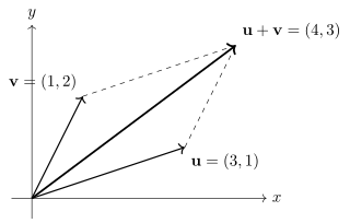
Diagram. Labels: x, y, mathbf u = (3,1), mathbf v = (1,2), mathbf u+mathbf v = (4,3)

The picture shows one rule at once: going along $\mathbf{u}$ and then $\mathbf{v}$ ends at the same corner as going along $\mathbf{v}$ and then $\mathbf{u}$ , so $\mathbf{u} + \mathbf{v} = \mathbf{v} + \mathbf{u}$ . Other rules are just as familiar. Scaling a sum is the same as adding the scaled arrows, $2(\mathbf{u} + \mathbf{v}) = 2\mathbf{u} + 2\mathbf{v}$ . Adding the zero arrow changes nothing, and every arrow is undone by its reverse.

Now look at polynomials of degree at most $2$ . We add them coefficient by coefficient, $(1 + 2x - x^2) + (3 - x + 4x^2) = 4 + x + 3x^2,$ and scale them the same way, $2(1 + 2x - x^2) = 2 + 4x - 2x^2$ . There is no picture of arrows here, yet the rules are identical: order does not matter in a sum, the zero polynomial changes nothing, and $-1 - 2x + x^2$ undoes $1 + 2x - x^2$ .

The same happens for $2 \times 2$ real matrices. Theorem 0.9.1 lists the rules for adding matrices and multiplying them by numbers, and they are again the same rules.

Arrows, polynomials and matrices are very different objects, but many arguments about them only use these rules. If we prove a statement from the rules alone, it holds for arrows, polynomials and matrices at once, and for every other system obeying the rules. So we list the rules once and give the systems that obey them a name.

A vector space is a set whose elements can be added and scaled by numbers from a field, with the usual rules of arithmetic.

1.1.2. The definition

Definition 1.1.1 (Vector Space)

Let $F$ be a field. A vector space over $F$ is a set $V$ together with two functions $+ \colon V \times V \to V, \ (\mathbf{u}, \mathbf{v}) \mapsto \mathbf{u} + \mathbf{v}, \qquad \cdot \colon F \times V \to V, \ (a, \mathbf{v}) \mapsto a\mathbf{v},$ called addition and scalar multiplication, such that the following axioms hold.

(VS1) $\mathbf{u} + \mathbf{v} = \mathbf{v} + \mathbf{u}$ for all $\mathbf{u}, \mathbf{v} \in V$ .
(VS2) $(\mathbf{u} + \mathbf{v}) + \mathbf{w} = \mathbf{u} + (\mathbf{v} + \mathbf{w})$ for all $\mathbf{u}, \mathbf{v}, \mathbf{w} \in V$ .
(VS3) There exists an element $\mathbf{0} \in V$ such that $\mathbf{v} + \mathbf{0} = \mathbf{v}$ for every $\mathbf{v} \in V$ .
(VS4) For every $\mathbf{v} \in V$ there exists an element $\mathbf{v}' \in V$ such that $\mathbf{v} + \mathbf{v}' = \mathbf{0}$ .
(VS5) $a(\mathbf{u} + \mathbf{v}) = a\mathbf{u} + a\mathbf{v}$ for all $a \in F$ and $\mathbf{u}, \mathbf{v} \in V$ .
(VS6) $(a + b)\mathbf{v} = a\mathbf{v} + b\mathbf{v}$ for all $a, b \in F$ and $\mathbf{v} \in V$ .
(VS7) $a(b\mathbf{v}) = (ab)\mathbf{v}$ for all $a, b \in F$ and $\mathbf{v} \in V$ .
(VS8) $1\mathbf{v} = \mathbf{v}$ for every $\mathbf{v} \in V$ , where $1$ is the identity element of $F$ .

Read the definition clause by clause.

The two functions. Addition takes two elements of $V$ and returns an element of $V$ . Scalar multiplication takes a number from $F$ and an element of $V$ and returns an element of $V$ . So “the sum stays in the set” and “a multiple stays in the set” are not extra axioms: they are built into the word “function into $V$ ”. When we test a candidate, this closure is the first thing to check.
(VS1)–(VS4) concern addition alone. It is commutative and associative, there is a vector $\mathbf{0}$ that changes nothing, and every vector can be undone. These are the axioms (F1)–(F4) of Definition 0.7.1, now for vectors.
(VS5) and (VS6) are the two distributive laws. In (VS6) the symbol $+$ appears twice with two meanings: on the left it adds scalars in $F$ , on the right it adds vectors in $V$ .
(VS7) says scaling by $b$ and then by $a$ is scaling by the product $ab$ , computed in $F$ .
(VS8) says the scalar $1$ acts as it should. It looks too obvious to state, but we will see below that it cannot be dropped.

Note the order of quantifiers in (VS3): one vector $\mathbf{0}$ works for every $\mathbf{v}$ . In (VS4) the vector $\mathbf{v}'$ is allowed to depend on $\mathbf{v}$ .

Definition 1.1.2 (Vectors and Scalars)

Let $V$ be a vector space over $F$ . The elements of $V$ are called vectors, and the elements of $F$ are called scalars. The element $\mathbf{0}$ in (VS3) is a zero vector of $V$ , and an element $\mathbf{v}'$ as in (VS4) is an additive inverse of $\mathbf{v}$ .

A vector space over $\mathbb{R}$ is also called a real vector space, and one over $\mathbb{C}$ a complex vector space. When the operations are clear from context, we say “ $V$ is a vector space over $F$ ” instead of naming the triple $(V, +, \cdot)$ . The field is part of the data, and we will see shortly that changing it changes the space.

We wrote “a zero vector” and “an additive inverse” on purpose. The axioms only say these exist. That there is only one of each is a theorem, proved later in this section.

Warning. Two different zeros. The scalar $0 \in F$ and the zero vector $\mathbf{0} \in V$ are different objects. In $M_2(\mathbb{R})$ , the scalar is the number $0$ and the zero vector is the zero matrix; in $\mathbb{R}^3$ , the zero vector is $(0, 0, 0)$ . This book writes the zero vector in bold. An equation such as $0\mathbf{v} = \mathbf{0}$ has a scalar on the left and a vector on the right, and mixing them up produces statements that make no sense, such as “ $\mathbf{v} = 0$ ” for a matrix $\mathbf{v}$ .

1.1.3. Examples

We start with the families we will use throughout the book. For each, the work is to say what the operations are and why the axioms hold. We check some axioms in full and point out the pattern for the rest.

Example (The Standard Vector Spaces)

Let $F$ be a field. Explain why each of the following is a vector space over $F$ .

(a) $F^n$ , with entrywise addition and scalar multiplication.
(b) $M_{m \times n}(F)$ , with the matrix operations of Definition 0.9.6 and Definition 0.9.7.
(c) $F[x]$ , with the addition of Definition 0.8.2 and $c \sum a_k x^k \mathrel{:=} \sum (c a_k) x^k$ .
(d) For a set $X$ , the set $F^X$ of all functions $X \to F$ , with the pointwise operations $(f + g)(t) \mathrel{:=} f(t) + g(t), \qquad (af)(t) \mathrel{:=} a f(t) \qquad \text{for all } t \in X.$
(e) The set $F^{\mathbb{N}}$ of all sequences $(s_0, s_1, s_2, \dots)$ of elements of $F$ , with termwise operations.

Solution.

(b) The sum and scalar multiple of $m \times n$ matrices are $m \times n$ matrices, so both operations are functions into $M_{m \times n}(F)$ . The eight axioms are exactly the rules of Theorem 0.9.1, with the zero matrix as $\mathbf{0}$ and $-\mathbf{A}$ as an additive inverse of $\mathbf{A}$ .
(c) Chapter 0 defines $F^n = M_{n \times 1}(F)$ , the column vectors, and the entrywise operations are the matrix operations. So (a) is the case of (b) with $n$ rows and $1$ column. The zero vector is $(0, \dots, 0)$ .
(d) The formulas define functions $f + g$ and $af$ from $X$ to $F$ , so the operations land in $F^X$ . Two functions $X \to F$ are equal when they take the same value at every $t \in X$ (Definition 0.4.1), so each axiom is checked one point at a time. For (VS3), let $\mathbf{0}$ be the zero function, $\mathbf{0}(t) = 0$ for all $t$ . Then $(f + \mathbf{0})(t) = f(t) + 0 = f(t)$ for every $t$ , by (F3), so $f + \mathbf{0} = f$ . For (VS4), let $f'(t) \mathrel{:=} -f(t)$ . Then $(f + f')(t) = f(t) + (-f(t)) = 0 = \mathbf{0}(t)$ by (F4), so $f + f' = \mathbf{0}$ . For (VS6), let $a, b \in F$ . For every $t \in X$ , $((a + b)f)(t) = (a + b)f(t) = af(t) + bf(t) = (af)(t) + (bf)(t) = (af + bf)(t),$ where the second equality is (F9) together with (F6) in $F$ . Hence $(a + b)f = af + bf$ . The other five axioms reduce in the same way to a field axiom at each point: (VS1) to (F1), (VS2) to (F2), (VS5) to (F9), (VS7) to (F5), and (VS8) to (F7) with (F6).
(e) A sequence $(s_0, s_1, \dots)$ is a function $\mathbb{N} \to F$ , $k \mapsto s_k$ , and the termwise operations are the pointwise ones. So (e) is (d) with $X = \mathbb{N}$ .
(f) Let $p = \sum a_k x^k \in F[x]$ and $c \in F$ . Only finitely many $a_k$ are non-zero, and $a_k = 0$ forces $c a_k = 0$ , so $cp$ is again a polynomial. The sum of polynomials is a polynomial by Definition 0.8.2. By Theorem 0.8.1 (parts 1 and 2), addition satisfies (VS1)–(VS4), with the zero polynomial as $\mathbf{0}$ and $-p$ as an additive inverse. Since polynomials are equal when their coefficients agree (Definition 0.8.1), (VS5)–(VS8) are checked coefficient by coefficient. For instance, the coefficient of $x^k$ in $(c + d)p$ is $(c + d)a_k = c a_k + d a_k$ , which is the coefficient of $x^k$ in $cp + dp$ . The others reduce in the same way: (VS5) to (F9), (VS7) to (F5), and (VS8) to (F7) with (F6).

The pattern is worth naming. Whenever the operations are defined entry by entry, point by point or coefficient by coefficient, each axiom for vectors is a field axiom applied in each slot. In fact (a), (b) and (e) are all instances of (d): a column in $F^n$ is a function $\{1, \dots, n\} \to F$ , and a matrix in $M_{m \times n}(F)$ is a function on the set of positions $\{1, \dots, m\} \times \{1, \dots, n\}$ .

A subset of a known space often works just as well, provided the operations do not lead out of it.

The set $F[x]_{\le n}$ of Definition 0.8.4 is a vector space over $F$ , with the operations of $F[x]$ . Closure is the only real issue. If $\deg p \le n$ and $\deg q \le n$ , then $\deg(p + q) \le \max(\deg p, \deg q) \le n$ by Theorem 0.8.2. If $a_k = 0$ for all $k > n$ , then $c a_k = 0$ for all $k > n$ , so $\deg(cp) \le n$ . The zero polynomial has degree $-\infty \le n$ , and $-p$ has the same coefficients as $p$ up to sign, so it stays in $F[x]_{\le n}$ . The six axioms (VS1), (VS2), (VS5)–(VS8) are equations that hold for all polynomials, so in particular for those of degree at most $n$ .

The next example applies the same pattern to a set of real numbers, with a smaller field of scalars.

Example (

\mathbb{Q}(\sqrt{2})

over

\mathbb{Q}

)

Let $\mathbb{Q}(\sqrt2) = \{ a + b\sqrt2 : a, b \in \mathbb{Q} \}$ , with the addition of $\mathbb{R}$ and with scalar multiplication $c(a + b\sqrt2) \mathrel{:=} ca + cb\sqrt2$ for $c \in \mathbb{Q}$ . Show that $\mathbb{Q}(\sqrt2)$ is a vector space over $\mathbb{Q}$ .

Solution. Let $\mathbf{u} = a + b\sqrt2$ and $\mathbf{v} = a' + b'\sqrt2$ with $a, b, a', b' \in \mathbb{Q}$ , and let $c \in \mathbb{Q}$ .

Closure. We have $\mathbf{u} + \mathbf{v} = (a + a') + (b + b')\sqrt2$ and $c\mathbf{u} = ca + cb\sqrt2$ . Sums and products of rationals are rational, so both lie in $\mathbb{Q}(\sqrt2)$ . Hence addition is a function $\mathbb{Q}(\sqrt2) \times \mathbb{Q}(\sqrt2) \to \mathbb{Q}(\sqrt2)$ , and scalar multiplication is a function $\mathbb{Q} \times \mathbb{Q}(\sqrt2) \to \mathbb{Q}(\sqrt2)$ .

Zero and additive inverses. The number $0 = 0 + 0\sqrt2$ lies in $\mathbb{Q}(\sqrt2)$ and satisfies $\mathbf{u} + 0 = \mathbf{u}$ , so (VS3) holds. The number $-\mathbf{u} = (-a) + (-b)\sqrt2$ lies in $\mathbb{Q}(\sqrt2)$ and satisfies $\mathbf{u} + (-\mathbf{u}) = 0$ , so (VS4) holds.

The identities. Scalar multiplication by $c \in \mathbb{Q}$ is the multiplication of real numbers, since $c(a + b\sqrt2) = ca + cb\sqrt2$ in $\mathbb{R}$ . So each of (VS1), (VS2) and (VS5)–(VS8) is an identity between real numbers, and it holds by the field axioms of $\mathbb{R}$ : (VS1) is (F1), (VS2) is (F2), (VS5) is (F9), (VS6) is (F9) with (F6), (VS7) is (F5), and (VS8) is (F7) with (F6). Hence $\mathbb{Q}(\sqrt2)$ is a vector space over $\mathbb{Q}$ .

We saw in Example ( $\mathbb{Q}(\sqrt{2})$ Is a Field) that $\mathbb{Q}(\sqrt2)$ is even a field. As a vector space over $\mathbb{Q}$ , we simply ignore how to multiply two of its elements together and keep only multiplication by rationals.

The same set can carry more than one field of scalars. The next example makes this concrete.

Example (The Same Set over Different Fields)

Explain why $\mathbb{C}$ is a vector space over $\mathbb{C}$ and also over $\mathbb{R}$ , and why $\mathbb{R}$ is a vector space over $\mathbb{R}$ and also over $\mathbb{Q}$ . In each case the addition is the usual one and the scalar multiplication is the usual product.

Solution. $\mathbb{C}$ over $\mathbb{C}$ is $F^1$ for $F = \mathbb{C}$ , covered by Example (The Standard Vector Spaces) (a). For $\mathbb{C}$ over $\mathbb{R}$ , a real number $r$ is the complex number $r + 0i$ , and $rz$ is their complex product, which lies in $\mathbb{C}$ . Each axiom is an identity among complex numbers in which some of the numbers happen to be real, so it holds by Proposition 0.6.1: (VS5) and (VS6) by distributivity together with commutativity, (VS7) by associativity of multiplication, and (VS8) since $1 \cdot z = z$ . The argument for $\mathbb{R}$ over $\mathbb{Q}$ is the same, with the field axioms of $\mathbb{R}$ in place of the laws of $\mathbb{C}$ .

As sets, $\mathbb{C}$ over $\mathbb{C}$ and $\mathbb{C}$ over $\mathbb{R}$ are the same. As vector spaces they differ, because the scalars available differ. In $\mathbb{C}$ over $\mathbb{C}$ , the vector $i$ is a scalar multiple of the vector $1$ . In $\mathbb{C}$ over $\mathbb{R}$ it is not, since $r \cdot 1 = i$ has no real solution $r$ . Later in this chapter this difference becomes a difference in dimension. That is why we always say over which field.

The degenerate case. The set $\{\mathbf{0}\}$ with one element, with $\mathbf{0} + \mathbf{0} = \mathbf{0}$ and $a\mathbf{0} = \mathbf{0}$ for every $a \in F$ , is a vector space over any field. Every axiom is an equation between elements that all equal $\mathbf{0}$ , and $\mathbf{0}$ serves as the zero vector and as its own additive inverse. It is called the zero space. It matters because it turns up constantly as an answer: the only solution of a system, or the smallest vector space inside every other one. Unlike a field, which must contain $1 \ne 0$ (Definition 0.7.1), a vector space is allowed to have a single element, since no axiom asks for a vector different from $\mathbf{0}$ .

A final example looks strange, but it satisfies every axiom.

Example (Positive Reals with Exotic Operations)

Let $V = \mathbb{R}_{>0} = \{ t \in \mathbb{R} : t > 0 \}$ . For $u, v \in V$ and $c \in \mathbb{R}$ , define $u \boxplus v \mathrel{:=} uv, \qquad c \boxdot v \mathrel{:=} v^{c}.$ Show that these operations are functions into $V$ , find the zero vector and the additive inverse of $v$ , and check (VS6) and (VS8).

Solution. Closure. For $u, v > 0$ and $c \in \mathbb{R}$ , the product $uv$ is positive and the power $v^{c}$ is positive. So $\boxplus \colon V \times V \to V$ and $\boxdot \colon \mathbb{R} \times V \to V$ .

(VS3). We need $z \in V$ with $v \boxplus z = v$ , that is, $vz = v$ , for every $v > 0$ . The number $z = 1$ works, since $v \cdot 1 = v$ . So the zero vector of $V$ is the real number $1$ .

(VS4). For $v \in V$ , we need $v' \in V$ with $v \boxplus v' = 1$ , that is, $vv' = 1$ . The number $v' = 1/v$ is positive and works. So the additive inverse of $v$ is $1/v$ .

(VS6). For $a, b \in \mathbb{R}$ and $v \in V$ , by the laws of exponents, $(a + b) \boxdot v = v^{a + b} = v^{a} v^{b} = (a \boxdot v) \boxplus (b \boxdot v).$

(VS8). $1 \boxdot v = v^{1} = v$ .

The remaining axioms (VS1), (VS2), (VS5) and (VS7) are Exercise (B3: Finishing the Positive Reals). So $V$ is a real vector space.

This example earns its place for one reason. The words “zero vector” and “addition” describe roles fixed by the axioms, not the familiar number $0$ or the familiar $+$ . Here the vector playing the role of $\mathbf{0}$ is the number $1$ , and “adding” means multiplying.

Quick check. Explain why each of the following, with the usual operations, is a vector space over $\mathbb{R}$ .

(a) The set $S$ of twice-differentiable functions $f \colon \mathbb{R} \to \mathbb{R}$ with $f'' + f = 0$ .
(b) The set of symmetric matrices $\mathbf{A} \in M_2(\mathbb{R})$ , that is, those with $\mathbf{A}^{\top} = \mathbf{A}$ .

Solution. Both are subsets of known spaces, so we use the pattern after Example (The Standard Vector Spaces): check closure, the zero vector and additive inverses; the other six axioms are identities inherited from the big space.

(a) $S \subseteq \mathbb{R}^{\mathbb{R}}$ . If $f, g \in S$ and $c \in \mathbb{R}$ , then by the sum and constant multiple rules of calculus, $f + g$ and $cf$ are twice differentiable, with $(f + g)'' + (f + g) = (f'' + f) + (g'' + g) = 0$ and $(cf)'' + cf = c(f'' + f) = 0$ . So both lie in $S$ . The zero function $\mathbf{0}$ satisfies $\mathbf{0}'' + \mathbf{0} = \mathbf{0}$ , so $\mathbf{0} \in S$ . If $f \in S$ , its additive inverse in $\mathbb{R}^{\mathbb{R}}$ is $t \mapsto -f(t)$ , and $-f(t) = (-1)f(t)$ by Theorem 0.7.1 (e); so it is the function $(-1)f$ , which lies in $S$ by closure under scaling. The identities hold in $\mathbb{R}^{\mathbb{R}}$ (Example (The Standard Vector Spaces) (d)), hence in $S$ . For instance $\sin$ and $\cos$ lie in $S$ .
(b) By Theorem 0.9.5, $(\mathbf{A} + \mathbf{B})^{\top} = \mathbf{A}^{\top} + \mathbf{B}^{\top} = \mathbf{A} + \mathbf{B}$ and $(c\mathbf{A})^{\top} = c\mathbf{A}^{\top} = c\mathbf{A}$ when $\mathbf{A}^{\top} = \mathbf{A}$ and $\mathbf{B}^{\top} = \mathbf{B}$ . The zero matrix is symmetric, and the additive inverse $-\mathbf{A}$ , which Chapter 0 defines as $(-1)\mathbf{A}$ , is symmetric by closure under scaling. The identities hold in $M_2(\mathbb{R})$ , hence for symmetric matrices.

1.1.4. Non-examples

Each non-example below is a small change to an example. We say what still works and name the exact clause that fails.

Change scalar multiplication on $\mathbb{R}^2$ to $c(x, y) \mathrel{:=} (cx, 0)$ , keeping the usual addition. Addition is untouched, so (VS1)–(VS4) hold. (VS5) holds: $c\big((x, y) + (x', y')\big) = (c(x + x'), 0) = (cx, 0) + (cx', 0)$ . In the same way (VS6) and (VS7) hold. But $1(0, 1) = (0, 0) \ne (0, 1)$ , so (VS8) fails.
Change the line $x + 2y = 0$ to $x + 2y = 3$ . Let $L = \{ (x, y) \in \mathbb{R}^2 : x + 2y = 3 \}$ with the operations of $\mathbb{R}^2$ . The points $(3, 0)$ and $(1, 1)$ lie on $L$ , but their sum $(4, 1)$ has $4 + 2 \cdot 1 = 6 \ne 3$ . So addition is not a function $L \times L \to L$ , and $L$ is not a vector space with these operations.
Change “degree at most $2$ ” to “degree exactly $2$ ”. In $\mathbb{R}[x]_{=2}$ (Definition 0.8.5), $x^2 + 2x$ and $-x^2 + 3$ have degree $2$ , but their sum $2x + 3$ has degree $1$ . Again addition leaves the set. There is no zero vector either: the zero polynomial has degree $-\infty$ , not $2$ .
Change the entries from real to integer, keeping $\mathbb{R}$ as the field. For $\mathbb{Z}^2 \subseteq \mathbb{R}^2$ , addition is fine, but $\tfrac12 (1, 0) = (\tfrac12, 0) \notin \mathbb{Z}^2$ . So scalar multiplication is not a function $\mathbb{R} \times \mathbb{Z}^2 \to \mathbb{Z}^2$ .

1.1.5. Why these axioms

Each axiom is there for a reason, and a few conventions deserve a comment.

(VS8) cannot be dropped. The first non-example satisfies all other axioms. Without (VS8), the “scalar multiplication” $c\mathbf{v} = \mathbf{0}$ for all $c$ and $\mathbf{v}$ would also be allowed, and scaling would carry no information at all.
(VS1) is in fact redundant. Commutativity of addition follows from the other seven axioms, by expanding $(1 + 1)(\mathbf{u} + \mathbf{v})$ in two ways (Exercise (C1: Commutativity Comes for Free)). It is kept because the proof is fiddly and nobody wants to repeat it.
Closure is not optional. Two of the non-examples fail only because an operation leads out of the set. That is why the definition asks for functions into $V$ .
The scalars form a field. We use division by non-zero scalars in the zero product law at the end of the next subsection. The warning after it shows what goes wrong without division.
The name. “Vector” originally meant an arrow in physics. The word is kept for elements of any vector space, even when they are polynomials or functions.

1.1.6. First consequences of the axioms

The definition says a zero vector and additive inverses exist, not that they are unique. Before writing $\mathbf{0}$ and $-\mathbf{v}$ as if each named one thing, we prove uniqueness. We also prove that familiar rules such as $0\mathbf{v} = \mathbf{0}$ follow from the axioms. None of this is obvious from the axioms: in Example (Positive Reals with Exotic Operations), $0 \boxdot v = v^0 = 1$ , which happens to be the zero vector there, and it takes a proof to see that this is no coincidence.

Throughout, we use one fact about functions without further comment: if two inputs are equal, the outputs are equal. So from $\mathbf{v} = \mathbf{w}$ we may conclude $\mathbf{u} + \mathbf{v} = \mathbf{u} + \mathbf{w}$ and $a\mathbf{v} = a\mathbf{w}$ .

The first tool lets us cancel a vector from both sides of an equation.

Theorem 1.1.1 (Left Cancellation Law)

Let $V$ be a vector space over $F$ and let $\mathbf{u}, \mathbf{v}, \mathbf{w} \in V$ . If $\mathbf{u} + \mathbf{v} = \mathbf{u} + \mathbf{w}$ , then $\mathbf{v} = \mathbf{w}$ .

Proof. Suppose $\mathbf{u} + \mathbf{v} = \mathbf{u} + \mathbf{w}$ . By (VS4) there is $\mathbf{u}' \in V$ with $\mathbf{u} + \mathbf{u}' = \mathbf{0}$ . Adding $\mathbf{u}'$ on the left of both sides gives $\mathbf{u}' + (\mathbf{u} + \mathbf{v}) = \mathbf{u}' + (\mathbf{u} + \mathbf{w})$ , and by (VS2), $(\mathbf{u}' + \mathbf{u}) + \mathbf{v} = (\mathbf{u}' + \mathbf{u}) + \mathbf{w}.$ By (VS1) and the choice of $\mathbf{u}'$ , $\mathbf{u}' + \mathbf{u} = \mathbf{u} + \mathbf{u}' = \mathbf{0}$ . Hence $\mathbf{0} + \mathbf{v} = \mathbf{0} + \mathbf{w}$ . By (VS1) this is $\mathbf{v} + \mathbf{0} = \mathbf{w} + \mathbf{0}$ , and by (VS3), $\mathbf{v} = \mathbf{w}$ .

Theorem 1.1.2 (Right Cancellation Law)

Let $V$ be a vector space over $F$ and let $\mathbf{u}, \mathbf{v}, \mathbf{w} \in V$ . If $\mathbf{v} + \mathbf{u} = \mathbf{w} + \mathbf{u}$ , then $\mathbf{v} = \mathbf{w}$ .

Proof. By (VS1), the hypothesis says $\mathbf{u} + \mathbf{v} = \mathbf{u} + \mathbf{w}$ . By Theorem 1.1.1, $\mathbf{v} = \mathbf{w}$ .

Uniqueness uses the standard move from Chapter 0: suppose there are two, and show they are equal.

Theorem 1.1.3 (Zero Vector Is Unique)

Let $V$ be a vector space over $F$ . There is exactly one element $\mathbf{0} \in V$ satisfying (VS3).

Proof. Existence is (VS3). Suppose $\mathbf{0}$ and $\mathbf{0}'$ both satisfy (VS3). Applying (VS3) for $\mathbf{0}'$ to the vector $\mathbf{0}$ , then (VS1), then (VS3) for $\mathbf{0}$ to the vector $\mathbf{0}'$ , $\mathbf{0} = \mathbf{0} + \mathbf{0}' = \mathbf{0}' + \mathbf{0} = \mathbf{0}'.$ This shows the zero vector is unique.

Theorem 1.1.4 (Additive Inverse Is Unique)

Let $V$ be a vector space over $F$ and $\mathbf{v} \in V$ . There is exactly one $\mathbf{v}' \in V$ with $\mathbf{v} + \mathbf{v}' = \mathbf{0}$ .

Proof. Existence is (VS4). Suppose $\mathbf{v} + \mathbf{v}' = \mathbf{0}$ and $\mathbf{v} + \mathbf{v}'' = \mathbf{0}$ . Then $\mathbf{v} + \mathbf{v}' = \mathbf{v} + \mathbf{v}''$ , and Theorem 1.1.1 gives $\mathbf{v}' = \mathbf{v}''$ .

Since the inverse is unique, it deserves a name.

Definition 1.1.3 (Notation for the Additive Inverse)

Let $V$ be a vector space over $F$ and $\mathbf{v} \in V$ . The unique additive inverse of $\mathbf{v}$ is denoted $-\mathbf{v}$ . For $\mathbf{u}, \mathbf{v} \in V$ we write $\mathbf{u} - \mathbf{v} \mathrel{:=} \mathbf{u} + (-\mathbf{v})$ .

For example, $\mathbf{v} + (-\mathbf{v}) = \mathbf{0}$ and $(-\mathbf{v}) + \mathbf{v} = \mathbf{0}$ by (VS1), so $\mathbf{v}$ is the additive inverse of $-\mathbf{v}$ . By Theorem 1.1.4, $-(-\mathbf{v}) = \mathbf{v}$ .

Remark. Axioms (VS1)–(VS4) say that $V$ with addition is an abelian group (Definition 0.10.1). So the four results above are also special cases of Theorem 0.10.1. We proved them directly to practice citing the axioms.

Now to scalars. No axiom mentions $0\mathbf{v}$ , so we must create a situation in which one applies. The move is to write the scalar $0$ in a fancy way, as $0 + 0$ , expand with a distributive law, and cancel. We will call it expand zero and cancel.

Theorem 1.1.5 (Zero Scalar Gives the Zero Vector)

Let $V$ be a vector space over $F$ . Then $0\mathbf{v} = \mathbf{0}$ for every $\mathbf{v} \in V$ .

Proof. Let $\mathbf{v} \in V$ . Since $0 + 0 = 0$ in $F$ by (F3), (VS6) gives $0\mathbf{v} + 0\mathbf{v} = (0 + 0)\mathbf{v} = 0\mathbf{v} = 0\mathbf{v} + \mathbf{0},$ where the last equality is (VS3). By Theorem 1.1.1, $0\mathbf{v} = \mathbf{0}$ .

The same move, with the zero vector in place of the zero scalar, handles $a\mathbf{0}$ .

Theorem 1.1.6 (Scalar Multiple of the Zero Vector)

Let $V$ be a vector space over $F$ . Then $a\mathbf{0} = \mathbf{0}$ for every $a \in F$ .

Proof. Let $a \in F$ . Since $\mathbf{0} + \mathbf{0} = \mathbf{0}$ by (VS3), (VS5) gives $a\mathbf{0} + a\mathbf{0} = a(\mathbf{0} + \mathbf{0}) = a\mathbf{0} = a\mathbf{0} + \mathbf{0},$ where the last equality is (VS3). By Theorem 1.1.1, $a\mathbf{0} = \mathbf{0}$ .

To identify a vector as $-\mathbf{v}$ , it is enough to show it adds with $\mathbf{v}$ to $\mathbf{0}$ , by Theorem 1.1.4. This gives the next two results.

Theorem 1.1.7 (Negation as Scalar Multiplication)

Let $V$ be a vector space over $F$ . Then $(-1)\mathbf{v} = -\mathbf{v}$ for every $\mathbf{v} \in V$ .

Proof. Let $\mathbf{v} \in V$ . By (VS8), (VS6), (F4) and Theorem 1.1.5, $\mathbf{v} + (-1)\mathbf{v} = 1\mathbf{v} + (-1)\mathbf{v} = (1 + (-1))\mathbf{v} = 0\mathbf{v} = \mathbf{0}.$ So $(-1)\mathbf{v}$ is an additive inverse of $\mathbf{v}$ , and by Theorem 1.1.4 it equals $-\mathbf{v}$ .

Theorem 1.1.8 (Negative Scalars)

Let $V$ be a vector space over $F$ . Then $(-a)\mathbf{v} = -(a\mathbf{v})$ for every $a \in F$ and $\mathbf{v} \in V$ .

Proof. Let $a \in F$ and $\mathbf{v} \in V$ . By (VS6), (F4) and Theorem 1.1.5, $a\mathbf{v} + (-a)\mathbf{v} = (a + (-a))\mathbf{v} = 0\mathbf{v} = \mathbf{0}.$ So $(-a)\mathbf{v}$ is an additive inverse of $a\mathbf{v}$ , and by Theorem 1.1.4 it equals $-(a\mathbf{v})$ .

The companion rules $a(-\mathbf{v}) = -(a\mathbf{v})$ and $a(\mathbf{u} - \mathbf{v}) = a\mathbf{u} - a\mathbf{v}$ are Exercise (B2: More Rules for Signs). From now on, we compute with $+$ , $-$ and scalars as in school algebra, citing these results when a step is not a single axiom.

The last result is the one we will use most. In a field, a product of non-zero numbers is non-zero (Theorem 0.7.1 (f)). The same holds for a scalar times a vector.

Theorem 1.1.9 (Zero Product Law)

Let $V$ be a vector space over $F$ , let $a \in F$ and $\mathbf{v} \in V$ . Then $a\mathbf{v} = \mathbf{0}$ if and only if $a = 0$ or $\mathbf{v} = \mathbf{0}$ .

Idea. The direction $(\Leftarrow)$ is the two zero results above, Theorem 1.1.5 and Theorem 1.1.6. For $(\Rightarrow)$ , the only way to get rid of $a$ is to multiply by $a^{-1}$ , and that is exactly where the hypothesis $a \ne 0$ and the field axiom (F8) are spent.

Proof. $(\Leftarrow)$ If $a = 0$ , then $a\mathbf{v} = \mathbf{0}$ by Theorem 1.1.5. If $\mathbf{v} = \mathbf{0}$ , then $a\mathbf{v} = \mathbf{0}$ by Theorem 1.1.6.

$(\Rightarrow)$ Suppose $a\mathbf{v} = \mathbf{0}$ . If $a = 0$ there is nothing to prove, so suppose $a \ne 0$ . By (F8), $a$ has an inverse $a^{-1} \in F$ . Then $\mathbf{v} = 1\mathbf{v} = (a^{-1}a)\mathbf{v} = a^{-1}(a\mathbf{v}) = a^{-1}\mathbf{0} = \mathbf{0},$ by (VS8), (F8) with (F6), (VS7), the hypothesis, and Theorem 1.1.6. This shows $a = 0$ or $\mathbf{v} = \mathbf{0}$ .

Warning. The zero product law needs division by scalars. Suppose we allowed integer “scalars” and let $V = \mathbb{F}_2 = \{0, 1\}$ with its own addition, where $n \cdot v$ is $v$ for odd $n$ and $0$ for even $n$ (for $n \ge 0$ this is $v + \dots + v$ with $n$ terms). Every rule of the shape (VS1)–(VS8) still holds. But $2 \cdot 1 = 1 + 1 = 0$ , although $2 \ne 0$ in $\mathbb{Z}$ and $1 \ne 0$ in $V$ . The proof above breaks exactly where it multiplies by $a^{-1}$ : the integer $2$ has no inverse in $\mathbb{Z}$ . This is one reason vector spaces are defined over a field.

As a first use, here is a fact about sizes. Let $\mathbf{v} \ne \mathbf{0}$ be a vector in a space over $\mathbb{R}$ . If $a\mathbf{v} = b\mathbf{v}$ , then $(a - b)\mathbf{v} = a\mathbf{v} - b\mathbf{v} = \mathbf{0}$ by (VS6) and Theorem 1.1.8, so $a = b$ by Theorem 1.1.9. So the multiples $a\mathbf{v}$ , $a \in \mathbb{R}$ , are all different, and a real vector space other than $\{\mathbf{0}\}$ has infinitely many elements (Exercise (C2: How Big Is a Vector Space?) treats a general field). This is our first glimpse of the question at the heart of this chapter: all these spaces are infinite sets, so how should we measure their size? The next section starts on the answer by looking at the vector spaces that sit inside a given one.

1.1.7. Exercises

A. Check your understanding

Exercise (A1)

(a) State the eight axioms of a vector space over a field $F$ , and say which of them involve scalars.
(b) Identify the zero vector in each of: $M_{2 \times 3}(\mathbb{R})$ ; $\mathbb{R}[x]_{\le 2}$ ; $\mathbb{R}^{\mathbb{R}}$ ; the space $\mathbb{R}_{>0}$ of Example (Positive Reals with Exotic Operations).
(c) True or false: a vector space can have exactly two elements. Justify your answer.
(d) True or false: in every vector space, $\mathbf{v} + \mathbf{v} = \mathbf{0}$ implies $\mathbf{v} = \mathbf{0}$ . Justify your answer.
(e) True or false: if $a\mathbf{v} = b\mathbf{v}$ and $\mathbf{v} \ne \mathbf{0}$ , then $a = b$ . Justify your answer.

Solution.

(a) See Definition 1.1.1. The axioms (VS5)–(VS8) involve scalars; (VS1)–(VS4) involve only addition.
(b) The zero matrix of size $2 \times 3$ ; the zero polynomial; the zero function $t \mapsto 0$ ; the number $1$ (Example (Positive Reals with Exotic Operations)).
(c) True. Let $F = \mathbb{F}_2$ . By Example (The Standard Vector Spaces) (a), $\mathbb{F}_2^1 = \mathbb{F}_2 = \{0, 1\}$ is a vector space over $\mathbb{F}_2$ , and it has exactly two elements.
(d) False. In the vector space $\mathbb{F}_2$ over $\mathbb{F}_2$ from (c), the vector $1 \ne 0$ satisfies $1 + 1 = 0$ . (Over $\mathbb{R}$ the statement is true: $\mathbf{v} + \mathbf{v} = (1 + 1)\mathbf{v} = 2\mathbf{v}$ by (VS8) and (VS6), and $2 \ne 0$ , so $\mathbf{v} = \mathbf{0}$ by Theorem 1.1.9.)
(e) True. By (VS6) and Theorem 1.1.8, $(a - b)\mathbf{v} = a\mathbf{v} + (-b)\mathbf{v} = a\mathbf{v} - b\mathbf{v} = \mathbf{0}$ . Since $\mathbf{v} \ne \mathbf{0}$ , Theorem 1.1.9 gives $a - b = 0$ , so $a = b$ .

B. Practice

Exercise (B1: Which Are Vector Spaces?)

Determine which of the following are vector spaces. Justify your answer.

(a) $\mathbb{R}^2$ over $\mathbb{R}$ , with the usual scalar multiplication but with addition $(x, y) + (x', y') \mathrel{:=} (x + x', 0)$ .
(b) The set of upper triangular matrices in $M_2(\mathbb{R})$ , over $\mathbb{R}$ , with the matrix operations.
(c) $\{ p \in \mathbb{R}[x] : p(1) = 0 \}$ , over $\mathbb{R}$ , with the operations of $\mathbb{R}[x]$ .
(d) $\{ p \in \mathbb{R}[x] : p(1) = 1 \}$ , over $\mathbb{R}$ , with the operations of $\mathbb{R}[x]$ .
(e) $\mathbb{R}^2$ over $\mathbb{C}$ , with $c(x, y) \mathrel{:=} (cx, cy)$ and the usual addition.

Solution.

(a) Not a vector space: (VS3) fails. Suppose $\mathbf{0} = (z_1, z_2)$ satisfied (VS3). Then $(0, 1) + (z_1, z_2) = (z_1, 0)$ would equal $(0, 1)$ , which is impossible since the second entries differ.
(b) A vector space. Let $\mathbf{A} = \begin{pmatrix} a & b \\ 0 & d \end{pmatrix}$ and $\mathbf{B} = \begin{pmatrix} a' & b' \\ 0 & d' \end{pmatrix}$ be upper triangular and $c \in \mathbb{R}$ . Then $\mathbf{A} + \mathbf{B} = \begin{pmatrix} a + a' & b + b' \\ 0 & d + d' \end{pmatrix}$ and $c\mathbf{A} = \begin{pmatrix} ca & cb \\ 0 & cd \end{pmatrix}$ are upper triangular, so the operations land in the set. The zero matrix is upper triangular, and so is $-\mathbf{A} = (-1)\mathbf{A}$ . The identities (VS1), (VS2), (VS5)–(VS8) hold for all matrices in $M_2(\mathbb{R})$ by Example (The Standard Vector Spaces) (b), hence for upper triangular ones.
(c) A vector space. Let $U = \{ p \in \mathbb{R}[x] : p(1) = 0 \}$ , $p, q \in U$ and $c \in \mathbb{R}$ . By Theorem 0.8.5, $(p + q)(1) = p(1) + q(1) = 0$ . Also $cp$ is the product of the constant polynomial $c$ with $p$ , since by the product formula of Definition 0.8.2 that product has coefficients $c a_k$ . So $(cp)(1) = c\, p(1) = 0$ . Hence $p + q, cp \in U$ . The zero polynomial has value $0$ at $1$ , and $-p = (-1)p \in U$ by closure under scaling. The identities hold in $\mathbb{R}[x]$ by Example (The Standard Vector Spaces) (c), hence in $U$ .
(d) Not a vector space: addition leaves the set. The constant polynomial $1$ lies in the set, but $(1 + 1)(1) = 2 \ne 1$ , so $1 + 1$ does not.
(e) Not a vector space: scalar multiplication leaves the set. We have $i \in \mathbb{C}$ and $(1, 0) \in \mathbb{R}^2$ , but $i(1, 0) = (i, 0) \notin \mathbb{R}^2$ . So the rule is not a function $\mathbb{C} \times \mathbb{R}^2 \to \mathbb{R}^2$ .

Exercise (B2: More Rules for Signs)

Let $V$ be a vector space over $F$ , let $a, b \in F$ and $\mathbf{u}, \mathbf{v} \in V$ . Prove that:

(a) $a(-\mathbf{v}) = -(a\mathbf{v})$ ;
(b) $(-a)(-\mathbf{v}) = a\mathbf{v}$ ;
(c) $a(\mathbf{u} - \mathbf{v}) = a\mathbf{u} - a\mathbf{v}$ and $(a - b)\mathbf{v} = a\mathbf{v} - b\mathbf{v}$ .

Hint: to show a vector equals $-(a\mathbf{v})$ , use Theorem 1.1.4.

Solution.

(a) By (VS5), (VS4) and Theorem 1.1.6, $a\mathbf{v} + a(-\mathbf{v}) = a(\mathbf{v} + (-\mathbf{v})) = a\mathbf{0} = \mathbf{0}.$ So $a(-\mathbf{v})$ is an additive inverse of $a\mathbf{v}$ . By Theorem 1.1.4, $a(-\mathbf{v}) = -(a\mathbf{v})$ .
(b) By (a) applied with the scalar $-a$ , then Theorem 1.1.8, then the remark after Definition 1.1.3, $(-a)(-\mathbf{v}) = -\big((-a)\mathbf{v}\big) = -\big(-(a\mathbf{v})\big) = a\mathbf{v}.$
(c) By Definition 1.1.3, (VS5) and (a), $a(\mathbf{u} - \mathbf{v}) = a(\mathbf{u} + (-\mathbf{v})) = a\mathbf{u} + a(-\mathbf{v}) = a\mathbf{u} + (-(a\mathbf{v})) = a\mathbf{u} - a\mathbf{v}.$ Similarly, since $a - b = a + (-b)$ in $F$ , (VS6) and Theorem 1.1.8 give $(a - b)\mathbf{v} = a\mathbf{v} + (-b)\mathbf{v} = a\mathbf{v} + (-(b\mathbf{v})) = a\mathbf{v} - b\mathbf{v}$ .

Exercise (B3: Finishing the Positive Reals)

Let $V = \mathbb{R}_{>0}$ with the operations $\boxplus$ and $\boxdot$ of Example (Positive Reals with Exotic Operations).

(a) Verify (VS1), (VS2), (VS5) and (VS7). Hence $V$ is a vector space over $\mathbb{R}$ .
(b) Compute the vector $(2 \boxdot 3) \boxplus \big((-1) \boxdot 6\big)$ .
(c) Find the vector $-(2 \boxdot 3)$ , and check your answer against Theorem 1.1.8.

Solution.

(a) Let $u, v, w \in V$ and $a, b \in \mathbb{R}$ . By the laws of real multiplication and of exponents for positive bases:
- (VS1): $u \boxplus v = uv = vu = v \boxplus u$ .
- (VS2): $(u \boxplus v) \boxplus w = (uv)w = u(vw) = u \boxplus (v \boxplus w)$ .
- (VS5): $a \boxdot (u \boxplus v) = (uv)^{a} = u^{a} v^{a} = (a \boxdot u) \boxplus (a \boxdot v)$ .
- (VS7): $a \boxdot (b \boxdot v) = (v^{b})^{a} = v^{ab} = (ab) \boxdot v$ .
Together with closure, (VS3), (VS4), (VS6) and (VS8) from Example (Positive Reals with Exotic Operations), all eight axioms hold. Hence $V$ is a vector space over $\mathbb{R}$ .
(b) $2 \boxdot 3 = 3^2 = 9$ and $(-1) \boxdot 6 = 6^{-1} = \tfrac16$ . So the vector is $9 \boxplus \tfrac16 = 9 \cdot \tfrac16 = \tfrac32$ .
(c) By Example (Positive Reals with Exotic Operations), the additive inverse of a vector $v$ is $1/v$ . Since $2 \boxdot 3 = 9$ , we get $-(2 \boxdot 3) = \tfrac19$ . By Theorem 1.1.8, this should equal $(-2) \boxdot 3 = 3^{-2} = \tfrac19$ , and it does.

C. Going deeper

Exercise (C1: Commutativity Comes for Free)

Let $V$ be a set with operations $+ \colon V \times V \to V$ and $\cdot \colon F \times V \to V$ satisfying (VS2)–(VS8), but not necessarily (VS1). Fix $\mathbf{0}$ as in (VS3).

(a) Let $\mathbf{v} \in V$ and $\mathbf{v}'$ as in (VS4). Put $\mathbf{w} = \mathbf{v}' + \mathbf{v}$ . Show that $\mathbf{w} + \mathbf{w} = \mathbf{w}$ , and deduce that $\mathbf{w} = \mathbf{0}$ .
(b) Show that $\mathbf{0} + \mathbf{v} = \mathbf{v}$ for every $\mathbf{v} \in V$ .
(c) Deduce that both cancellation laws hold: $\mathbf{u} + \mathbf{v} = \mathbf{u} + \mathbf{w}$ implies $\mathbf{v} = \mathbf{w}$ , and $\mathbf{v} + \mathbf{u} = \mathbf{w} + \mathbf{u}$ implies $\mathbf{v} = \mathbf{w}$ .
(d) By expanding $(1 + 1)(\mathbf{u} + \mathbf{v})$ in two ways, prove that $\mathbf{u} + \mathbf{v} = \mathbf{v} + \mathbf{u}$ for all $\mathbf{u}, \mathbf{v} \in V$ .

Hint: in (a), add an additive inverse of $\mathbf{w}$ on the right. The proof of Theorem 1.1.1 used (VS1), so it cannot be quoted in (c).

Solution. Throughout we use only (VS2)–(VS8), and we drop brackets in sums whenever (VS2) allows it.

(a) Since $\mathbf{v} + \mathbf{v}' = \mathbf{0}$ and $\mathbf{v}' + \mathbf{0} = \mathbf{v}'$ by (VS3), $\mathbf{w} + \mathbf{w} = \mathbf{v}' + (\mathbf{v} + \mathbf{v}') + \mathbf{v} = \mathbf{v}' + \mathbf{0} + \mathbf{v} = \mathbf{v}' + \mathbf{v} = \mathbf{w}.$ By (VS4) choose $\mathbf{w}'$ with $\mathbf{w} + \mathbf{w}' = \mathbf{0}$ . Adding $\mathbf{w}'$ on the right of $\mathbf{w} + \mathbf{w} = \mathbf{w}$ gives $\mathbf{w} + (\mathbf{w} + \mathbf{w}') = \mathbf{w} + \mathbf{w}'$ , that is, $\mathbf{w} + \mathbf{0} = \mathbf{0}$ . By (VS3), $\mathbf{w} = \mathbf{0}$ . So $\mathbf{v}' + \mathbf{v} = \mathbf{0}$ as well.
(b) Let $\mathbf{v} \in V$ and $\mathbf{v}'$ as in (VS4). By (a), (VS2) and (VS3), $\mathbf{0} + \mathbf{v} = (\mathbf{v} + \mathbf{v}') + \mathbf{v} = \mathbf{v} + (\mathbf{v}' + \mathbf{v}) = \mathbf{v} + \mathbf{0} = \mathbf{v}.$
(c) Suppose $\mathbf{u} + \mathbf{v} = \mathbf{u} + \mathbf{w}$ , and let $\mathbf{u}'$ be as in (VS4). Adding $\mathbf{u}'$ on the left and using (VS2), $(\mathbf{u}' + \mathbf{u}) + \mathbf{v} = (\mathbf{u}' + \mathbf{u}) + \mathbf{w}$ . By (a), $\mathbf{u}' + \mathbf{u} = \mathbf{0}$ , so $\mathbf{0} + \mathbf{v} = \mathbf{0} + \mathbf{w}$ , and (b) gives $\mathbf{v} = \mathbf{w}$ . Now suppose $\mathbf{v} + \mathbf{u} = \mathbf{w} + \mathbf{u}$ . Adding $\mathbf{u}'$ on the right and using (VS2), $\mathbf{v} + (\mathbf{u} + \mathbf{u}') = \mathbf{w} + (\mathbf{u} + \mathbf{u}')$ , so $\mathbf{v} + \mathbf{0} = \mathbf{w} + \mathbf{0}$ , and (VS3) gives $\mathbf{v} = \mathbf{w}$ .
(d) Let $\mathbf{u}, \mathbf{v} \in V$ . On the one hand, by (VS6) and (VS8), $(1 + 1)(\mathbf{u} + \mathbf{v}) = 1(\mathbf{u} + \mathbf{v}) + 1(\mathbf{u} + \mathbf{v}) = \mathbf{u} + \mathbf{v} + \mathbf{u} + \mathbf{v}.$ On the other hand, by (VS5), then (VS6) and (VS8), $(1 + 1)(\mathbf{u} + \mathbf{v}) = (1 + 1)\mathbf{u} + (1 + 1)\mathbf{v} = \mathbf{u} + \mathbf{u} + \mathbf{v} + \mathbf{v}.$ Hence $\mathbf{u} + (\mathbf{v} + \mathbf{u}) + \mathbf{v} = \mathbf{u} + (\mathbf{u} + \mathbf{v}) + \mathbf{v}$ , grouping by (VS2). Canceling $\mathbf{u}$ on the left and then $\mathbf{v}$ on the right, by (c), gives $\mathbf{v} + \mathbf{u} = \mathbf{u} + \mathbf{v}$ . This proves (VS1).

Exercise (C2: How Big Is a Vector Space?)

(a) Let $F$ be an infinite field and $V \ne \{\mathbf{0}\}$ a vector space over $F$ . Prove that $V$ is an infinite set.
(b) Let $p$ be a prime and $n \ge 1$ . How many elements does the vector space $\mathbb{F}_p^n$ over $\mathbb{F}_p$ have? Explain why this does not contradict (a).

Hint: for (a), fix $\mathbf{v} \ne \mathbf{0}$ and consider the function $F \to V$ , $a \mapsto a\mathbf{v}$ .

Solution.

(a) Since $V \ne \{\mathbf{0}\}$ and $\mathbf{0} \in V$ , there is $\mathbf{v} \in V$ with $\mathbf{v} \ne \mathbf{0}$ . Consider $\varphi \colon F \to V$ , $\varphi(a) = a\mathbf{v}$ . Suppose $\varphi(a) = \varphi(b)$ , so $a\mathbf{v} = b\mathbf{v}$ . By Exercise (B2: More Rules for Signs) (c), $(a - b)\mathbf{v} = a\mathbf{v} - b\mathbf{v} = \mathbf{0}$ . Since $\mathbf{v} \ne \mathbf{0}$ , Theorem 1.1.9 gives $a - b = 0$ , so $a = b$ . Therefore $\varphi$ is injective. An injective function from an infinite set has an infinite image, so $V$ , which contains the image of $\varphi$ , is infinite.
(b) An element of $\mathbb{F}_p^n$ is a list $(x_1, \dots, x_n)$ with each $x_i$ chosen freely from the $p$ elements of $\mathbb{F}_p$ . So $\mathbb{F}_p^n$ has $p^n$ elements. There is no contradiction, because (a) assumes the field is infinite and $\mathbb{F}_p$ is finite. The proof of (a) still shows that $a \mapsto a\mathbf{v}$ is injective, so a non-zero space over $\mathbb{F}_p$ has at least $p$ elements.

Exercise (C3: Shrinking the Field)

Let $F$ be a field and let $K \subseteq F$ be a subset with $0, 1 \in K$ that is closed under addition, multiplication, negatives, and inverses of non-zero elements. (So $K$ is itself a field with the operations of $F$ ; for example $\mathbb{Q} \subseteq \mathbb{R} \subseteq \mathbb{C}$ .)

(a) Let $V$ be a vector space over $F$ . Prove that $V$ , with the same addition and with scalar multiplication restricted to $K \times V$ , is a vector space over $K$ .
(b) Deduce that $\mathbb{C}^n$ is a vector space over $\mathbb{R}$ and over $\mathbb{Q}$ .
(c) Explain why $\mathbb{R}$ , with its usual addition and multiplication, is not a vector space over $\mathbb{C}$ .

Solution.

(a) The addition is unchanged, so it is a function $V \times V \to V$ satisfying (VS1)–(VS4). Scalar multiplication $F \times V \to V$ restricts to a function $K \times V \to V$ , since $K \subseteq F$ . The axioms (VS5)–(VS7) are statements about all scalars in $F$ , so they hold in particular for all scalars in $K$ ; the operations $a + b$ and $ab$ appearing in them are the same in $K$ as in $F$ . For (VS8), the identity of $K$ is the identity $1$ of $F$ , and $1\mathbf{v} = \mathbf{v}$ holds in $V$ over $F$ . Hence $V$ is a vector space over $K$ .
(b) $\mathbb{C}^n$ is a vector space over $\mathbb{C}$ by Example (The Standard Vector Spaces) (a). The subsets $\mathbb{R} \subseteq \mathbb{C}$ and $\mathbb{Q} \subseteq \mathbb{C}$ contain $0$ and $1$ and are closed under the four operations, so (a) applies to both.
(c) The only candidate for scalar multiplication is $(c, t) \mapsto ct$ , the product in $\mathbb{C}$ . But it does not land in $\mathbb{R}$ : $i \in \mathbb{C}$ and $1 \in \mathbb{R}$ , while $i \cdot 1 = i \notin \mathbb{R}$ . So there is no function $\mathbb{C} \times \mathbb{R} \to \mathbb{R}$ given by this rule, and $\mathbb{R}$ is not a vector space over $\mathbb{C}$ with these operations.