4.2 Change of Basis and Similarity

The matrix $[T]_{\mathcal{B}}^{\mathcal{C}}$ of a linear map depends on two choices of basis, and different choices can give very different matrices for the same map. This section answers two questions left open by that fact. How are two matrices of the same map related? And which properties of a matrix belong to the map itself, so that no choice of basis can change them? The answers are the change-of-basis formula, drawn as a commutative square, and the relation of similarity.

4.2.1. Change-of-coordinates matrices

Recall the definition of the matrix of a map (Definition 4.1.1). If $\mathcal{B} = (\mathbf{v}_1, \dots, \mathbf{v}_n)$ is a basis of $V$ and $\mathcal{C}$ is a basis of $W$ , then $[T]_{\mathcal{B}}^{\mathcal{C}}$ is the matrix whose $j$ -th column is $[T\mathbf{v}_j]_{\mathcal{C}}$ , and it turns coordinates into coordinates: $[T\mathbf{v}]_{\mathcal{C}} = [T]_{\mathcal{B}}^{\mathcal{C}}[\mathbf{v}]_{\mathcal{B}}$ (Theorem 4.1.1).

Recall the reflection from the previous section (Example (A Reflection in Two Bases)), which motivates this one. Let $R \colon \mathbb{R}^2 \to \mathbb{R}^2$ be the reflection across the line $y = x$ , so $R(x, y) = (y, x)$ . In the standard basis $\mathcal{E} = (\mathbf{e}_1, \mathbf{e}_2)$ , we have $R\mathbf{e}_1 = \mathbf{e}_2$ and $R\mathbf{e}_2 = \mathbf{e}_1$ , so $[R]_{\mathcal{E}}^{\mathcal{E}} = \begin{pmatrix} 0 & 1 \\ 1 & 0 \end{pmatrix}.$ Now use the basis $\mathcal{B} = ((1, 1), (1, -1))$ , one vector on the mirror line and one perpendicular to it. Then $R(1, 1) = (1, 1)$ and $R(1, -1) = (-1, 1) = -(1, -1)$ , so $[R]_{\mathcal{B}}^{\mathcal{B}} = \begin{pmatrix} 1 & 0 \\ 0 & -1 \end{pmatrix}.$ The second matrix shows at a glance what $R$ does: it keeps one direction and flips the other. The two matrices describe the same map, so there must be a rule converting one into the other. The first step is to convert the coordinates of a single vector.

Take $\mathbf{v} = (3, 1)$ . Its standard coordinates are $[\mathbf{v}]_{\mathcal{E}} = (3, 1)$ . In the basis $\mathcal{B}$ , we solve $a(1, 1) + b(1, -1) = (3, 1)$ , which gives $a = 2$ , $b = 1$ , so $[\mathbf{v}]_{\mathcal{B}} = (2, 1)$ . The same vector has two different coordinate columns, and we want a matrix that translates between them. Since the identity map $\operatorname{id}_V$ sends every vector to itself, the matrix of $\operatorname{id}_V$ , with one basis on the input side and the other on the output side, should do exactly this job.

A change-of-coordinates matrix is the matrix of “do nothing”, read with one basis on the way in and another on the way out.

Definition 4.2.1 (Change-of-coordinates matrix)

Let $V$ be a finite-dimensional vector space over $F$ , and let $\mathcal{B} = (\mathbf{v}_1, \dots, \mathbf{v}_n)$ and $\mathcal{C}$ be ordered bases of $V$ . The change-of-coordinates matrix from $\mathcal{B}$ to $\mathcal{C}$ is the $n \times n$ matrix $[\operatorname{id}]_{\mathcal{B}}^{\mathcal{C}} \mathrel{:=} [\operatorname{id}_V]_{\mathcal{B}}^{\mathcal{C}},$ the matrix of the identity map $\operatorname{id}_V \colon V \to V$ with respect to the input basis $\mathcal{B}$ and the output basis $\mathcal{C}$ . Its $j$ -th column is $[\mathbf{v}_j]_{\mathcal{C}}$ .

In words: to build $[\operatorname{id}]_{\mathcal{B}}^{\mathcal{C}}$ , take the vectors of the old basis $\mathcal{B}$ one at a time, write each in the new basis $\mathcal{C}$ , and put the coordinate columns side by side. The column description is Definition 4.1.1 with $T = \operatorname{id}_V$ , since $\operatorname{id}_V(\mathbf{v}_j) = \mathbf{v}_j$ . Both bases must be bases of the same space $V$ , and both are ordered: reordering either one permutes the columns or the rows.

Examples.

Into the standard basis of $F^n$ . If $\mathcal{B} = (\mathbf{b}_1, \dots, \mathbf{b}_n)$ is a basis of $F^n$ and $\mathcal{E}$ is the standard basis, then $[\mathbf{b}_j]_{\mathcal{E}} = \mathbf{b}_j$ . So $[\operatorname{id}]_{\mathcal{B}}^{\mathcal{E}}$ is the matrix whose columns are the vectors of $\mathcal{B}$ themselves. For $\mathcal{B} = ((1, 1), (1, -1))$ in $\mathbb{R}^2$ , $[\operatorname{id}]_{\mathcal{B}}^{\mathcal{E}} = \begin{pmatrix} 1 & 1 \\ 1 & -1 \end{pmatrix}$ , and indeed $\begin{pmatrix} 1 & 1 \\ 1 & -1 \end{pmatrix} \begin{pmatrix} 2 \\ 1 \end{pmatrix} = \begin{pmatrix} 3 \\ 1 \end{pmatrix}$ turns $[\mathbf{v}]_{\mathcal{B}}$ into $[\mathbf{v}]_{\mathcal{E}}$ for $\mathbf{v} = (3, 1)$ .
Out of the standard basis. In the other direction, $[\operatorname{id}]_{\mathcal{E}}^{\mathcal{B}}$ has columns $[\mathbf{e}_1]_{\mathcal{B}}$ and $[\mathbf{e}_2]_{\mathcal{B}}$ . Solving $a(1, 1) + b(1, -1) = (1, 0)$ gives $a = b = \frac12$ , and solving for $(0, 1)$ gives $a = \frac12$ , $b = -\frac12$ . So $[\operatorname{id}]_{\mathcal{E}}^{\mathcal{B}} = \frac12 \begin{pmatrix} 1 & 1 \\ 1 & -1 \end{pmatrix}$ . This is the inverse of the previous matrix, which the next theorem explains.
Polynomials. In $F[x]_{\le 2}$ , let $\mathcal{B} = (1, x, x^2)$ and $\mathcal{C} = (1, x - 1, (x - 1)^2)$ . Expanding $(x - 1)^2 = 1 - 2x + x^2$ , the vectors of $\mathcal{C}$ have $\mathcal{B}$ -coordinates $(1, 0, 0)$ , $(-1, 1, 0)$ and $(1, -2, 1)$ , so $[\operatorname{id}]_{\mathcal{C}}^{\mathcal{B}} = \begin{pmatrix} 1 & -1 & 1 \\ 0 & 1 & -2 \\ 0 & 0 & 1 \end{pmatrix}.$
Degenerate case. If $\mathcal{C} = \mathcal{B}$ , then $[\mathbf{v}_j]_{\mathcal{B}} = \mathbf{e}_j$ , so $[\operatorname{id}]_{\mathcal{B}}^{\mathcal{B}} = \mathbf{I}_n$ . Changing nothing is recorded by the identity matrix, as it should be.

Non-example by minimal change. Replace the basis $((1, 1), (1, -1))$ by the list $\mathcal{L} = ((1, 1), (2, 2))$ . We can still write the matrix with these vectors as columns, but $\mathcal{L}$ is not a basis, so “coordinates with respect to $\mathcal{L}$ ” are not defined: $(2, 2) = 2(1, 1) + 0(2, 2) = 0(1, 1) + 1(2, 2)$ has two coordinate columns, and $(1, 0)$ has none. The clause that fails is “ $\mathcal{B}$ is a basis”, which Definition 1.5.2 needs for coordinates to exist and be unique.

Warning. Watch the direction. The columns of $[\operatorname{id}]_{\mathcal{B}}^{\mathcal{C}}$ are the $\mathcal{B}$ -vectors written in $\mathcal{C}$ , and the matrix turns $\mathcal{B}$ -coordinates into $\mathcal{C}$ -coordinates. Using it the other way gives nonsense. With $\mathcal{B} = ((1, 1), (1, -1))$ , the matrix $\begin{pmatrix} 1 & 1 \\ 1 & -1 \end{pmatrix} = [\operatorname{id}]_{\mathcal{B}}^{\mathcal{E}}$ applied to $[\mathbf{v}]_{\mathcal{E}} = (3, 1)$ gives $(4, 2)$ , which is not $[\mathbf{v}]_{\mathcal{B}} = (2, 1)$ . A reliable test: the first column must be the first input basis vector written in the output basis. Here $(1, 1) = 1 \cdot \mathbf{e}_1 + 1 \cdot \mathbf{e}_2$ , so the column $(1, 1)$ belongs to $[\operatorname{id}]_{\mathcal{B}}^{\mathcal{E}}$ , which accepts $\mathcal{B}$ -coordinates.

The examples suggest three facts: the matrix converts coordinates, converting twice multiplies the matrices, and converting back inverts the matrix. All three follow from results about matrices of maps, applied to the identity.

Theorem 4.2.1 (Change of Coordinates)

Let $V$ be a vector space of dimension $n$ , and let $\mathcal{B}$ , $\mathcal{C}$ , $\mathcal{D}$ be bases of $V$ .

(a) For every $\mathbf{v} \in V$ , $[\mathbf{v}]_{\mathcal{C}} = [\operatorname{id}]_{\mathcal{B}}^{\mathcal{C}}[\mathbf{v}]_{\mathcal{B}}$ . Moreover, $[\operatorname{id}]_{\mathcal{B}}^{\mathcal{C}}$ is the only matrix $M \in M_n(F)$ with $[\mathbf{v}]_{\mathcal{C}} = M[\mathbf{v}]_{\mathcal{B}}$ for every $\mathbf{v} \in V$ .
(b) $[\operatorname{id}]_{\mathcal{B}}^{\mathcal{D}} = [\operatorname{id}]_{\mathcal{C}}^{\mathcal{D}}[\operatorname{id}]_{\mathcal{B}}^{\mathcal{C}}$ .
(c) $[\operatorname{id}]_{\mathcal{B}}^{\mathcal{C}}$ is invertible, and $\big([\operatorname{id}]_{\mathcal{B}}^{\mathcal{C}}\big)^{-1} = [\operatorname{id}]_{\mathcal{C}}^{\mathcal{B}}$ .

Proof.

(a) Apply Theorem 4.1.1, including its uniqueness clause, to $\operatorname{id}_V$ with input basis $\mathcal{B}$ and output basis $\mathcal{C}$ : since $\operatorname{id}_V(\mathbf{v}) = \mathbf{v}$ , it says $[\mathbf{v}]_{\mathcal{C}} = [\operatorname{id}]_{\mathcal{B}}^{\mathcal{C}}[\mathbf{v}]_{\mathcal{B}}$ for every $\mathbf{v}$ , and that no other matrix has this property.
(b) Since $\operatorname{id}_V = \operatorname{id}_V \circ \operatorname{id}_V$ , Theorem 4.1.2, with $\mathcal{B}$ on the input, $\mathcal{C}$ in the middle and $\mathcal{D}$ on the output, gives $[\operatorname{id}]_{\mathcal{B}}^{\mathcal{D}} = [\operatorname{id}]_{\mathcal{C}}^{\mathcal{D}}[\operatorname{id}]_{\mathcal{B}}^{\mathcal{C}}$ .
(c) Taking $\mathcal{D} = \mathcal{B}$ in (b) gives $[\operatorname{id}]_{\mathcal{C}}^{\mathcal{B}}[\operatorname{id}]_{\mathcal{B}}^{\mathcal{C}} = [\operatorname{id}]_{\mathcal{B}}^{\mathcal{B}} = \mathbf{I}_n$ , where the last equality holds because, writing $\mathcal{B} = (\mathbf{v}_1, \dots, \mathbf{v}_n)$ , the $j$ -th column of $[\operatorname{id}]_{\mathcal{B}}^{\mathcal{B}}$ is $[\mathbf{v}_j]_{\mathcal{B}} = \mathbf{e}_j$ . Swapping the roles of $\mathcal{B}$ and $\mathcal{C}$ gives $[\operatorname{id}]_{\mathcal{B}}^{\mathcal{C}}[\operatorname{id}]_{\mathcal{C}}^{\mathcal{B}} = \mathbf{I}_n$ . By Definition 0.9.13, $[\operatorname{id}]_{\mathcal{B}}^{\mathcal{C}}$ is invertible with inverse $[\operatorname{id}]_{\mathcal{C}}^{\mathcal{B}}$ .

So every change-of-coordinates matrix is invertible. The converse is also true, and it will matter when we compare matrices: every invertible matrix is a change-of-coordinates matrix, for a suitable new basis.

Proposition 4.2.2 (Invertible matrices are changes of basis)

Let $\mathcal{B} = (\mathbf{v}_1, \dots, \mathbf{v}_n)$ be a basis of $V$ , and let $\mathbf{P} = (p_{ij}) \in M_n(F)$ be invertible. Put $\mathbf{v}_j' \mathrel{:=} p_{1j}\mathbf{v}_1 + p_{2j}\mathbf{v}_2 + \dots + p_{nj}\mathbf{v}_n \qquad (j = 1, \dots, n).$ Then $\mathcal{B}' = (\mathbf{v}_1', \dots, \mathbf{v}_n')$ is a basis of $V$ , and $[\operatorname{id}]_{\mathcal{B}'}^{\mathcal{B}} = \mathbf{P}$ .

Proof. By Definition 1.5.2, $[\mathbf{v}_j']_{\mathcal{B}}$ is the $j$ -th column $\mathbf{p}_j$ of $\mathbf{P}$ . Let $c_1, \dots, c_n \in F$ satisfy $c_1\mathbf{v}_1' + \dots + c_n\mathbf{v}_n' = \mathbf{0}$ . Taking $\mathcal{B}$ -coordinates and using Theorem 1.5.2, $c_1\mathbf{p}_1 + \dots + c_n\mathbf{p}_n = [\mathbf{0}]_{\mathcal{B}} = \mathbf{0},$ that is, $\mathbf{P}\mathbf{c} = \mathbf{0}$ with $\mathbf{c} = (c_1, \dots, c_n)$ , by Theorem 0.9.3. Since $\mathbf{P}$ is invertible, Theorem 3.4.4 ((a) $\Rightarrow$ (b)) gives $\mathbf{c} = \mathbf{0}$ . So $\mathcal{B}'$ is linearly independent. It has length $n = \dim V$ , hence it is a basis by Theorem 1.6.4 (a). Finally, the $j$ -th column of $[\operatorname{id}]_{\mathcal{B}'}^{\mathcal{B}}$ is $[\mathbf{v}_j']_{\mathcal{B}} = \mathbf{p}_j$ , so $[\operatorname{id}]_{\mathcal{B}'}^{\mathcal{B}} = \mathbf{P}$ .

Example (Coordinates around the point

1

)

In $\mathbb{R}[x]_{\le 2}$ , let $\mathcal{B} = (1, x, x^2)$ and $\mathcal{C} = (1, x - 1, (x - 1)^2)$ . Find $[\operatorname{id}]_{\mathcal{B}}^{\mathcal{C}}$ , and use it to write $p = 2 + 3x + x^2$ in powers of $x - 1$ .

Solution. From the examples above, $[\operatorname{id}]_{\mathcal{C}}^{\mathcal{B}} = \begin{pmatrix} 1 & -1 & 1 \\ 0 & 1 & -2 \\ 0 & 0 & 1 \end{pmatrix}$ . By Theorem 4.2.1 (c), $[\operatorname{id}]_{\mathcal{B}}^{\mathcal{C}}$ is its inverse. We can also read it off directly: $1 = 1$ , $x = 1 + (x - 1)$ , and $x^2 = (1 + (x - 1))^2 = 1 + 2(x - 1) + (x - 1)^2$ . So $[\operatorname{id}]_{\mathcal{B}}^{\mathcal{C}} = \begin{pmatrix} 1 & 1 & 1 \\ 0 & 1 & 2 \\ 0 & 0 & 1 \end{pmatrix},$ and multiplying the two matrices gives $\mathbf{I}_3$ , as the theorem predicts. By Theorem 4.2.1 (a), $[p]_{\mathcal{C}} = \begin{pmatrix} 1 & 1 & 1 \\ 0 & 1 & 2 \\ 0 & 0 & 1 \end{pmatrix} \begin{pmatrix} 2 \\ 3 \\ 1 \end{pmatrix} = \begin{pmatrix} 6 \\ 5 \\ 1 \end{pmatrix}.$ Hence $2 + 3x + x^2 = 6 + 5(x - 1) + (x - 1)^2$ . Check at $x = 1$ : both sides equal $6$ . The $\mathcal{C}$ -coordinates are $p(1)$ , $p'(1)$ and $p''(1)/2$ , the Taylor coefficients at $1$ .

4.2.2. Change of basis for linear maps

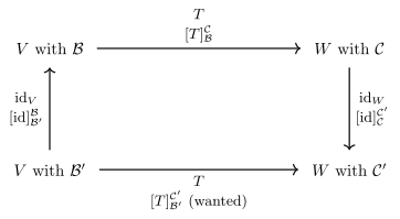
Now return to a linear map $T \colon V \to W$ between finite-dimensional spaces. Suppose we know its matrix $[T]_{\mathcal{B}}^{\mathcal{C}}$ and want the matrix $[T]_{\mathcal{B}'}^{\mathcal{C}'}$ for new bases $\mathcal{B}'$ of $V$ and $\mathcal{C}'$ of $W$ . The trick is to write $T$ in a slightly more elaborate way that does nothing: $T = \operatorname{id}_W \circ T \circ \operatorname{id}_V .$ Each factor can now carry its own pair of bases, and the matrix of the composite is the product of the matrices. The picture keeps track of which basis sits where.

$Diagram. Labels: T\\[1pt] mtx TsB sC, T\\[1pt] mtx TsB 'sC ' (wanted), id_V\\[1pt] mtx id sB 'sB, id_W\\[1pt] mtx id sC sC ', V with sB, W with sC, V with sB ', W with sC '$

Going along the bottom edge applies $T$ . Going up, across the top and down applies $\operatorname{id}_W \circ T \circ \operatorname{id}_V$ , which is the same map. So the two routes must have the same matrix. Reading the long route, the step done first (up the left side) is written on the right.

Theorem 4.2.3 (Change of Basis for Linear Maps)

Let $V$ and $W$ be finite-dimensional vector spaces over $F$ , let $\mathcal{B}, \mathcal{B}'$ be bases of $V$ and $\mathcal{C}, \mathcal{C}'$ bases of $W$ , and let $T \colon V \to W$ be linear. Then $[T]_{\mathcal{B}'}^{\mathcal{C}'} = [\operatorname{id}]_{\mathcal{C}}^{\mathcal{C}'}\,[T]_{\mathcal{B}}^{\mathcal{C}}\,[\operatorname{id}]_{\mathcal{B}'}^{\mathcal{B}}.$ In particular, for an operator $T \in \mathcal{L}(V)$ and bases $\mathcal{B}, \mathcal{B}'$ of $V$ , with $\mathbf{P} = [\operatorname{id}]_{\mathcal{B}'}^{\mathcal{B}}$ , $[T]_{\mathcal{B}'}^{\mathcal{B}'} = \mathbf{P}^{-1}\,[T]_{\mathcal{B}}^{\mathcal{B}}\,\mathbf{P} .$

Idea. Nothing is computed: the formula is the change-of-basis square read along its long route. ① Write $T = \operatorname{id}_W \circ T \circ \operatorname{id}_V$ . ② Give the middle factor the bases whose matrix we know. ③ Apply the composition rule twice. Do not memorize the formula; redraw the square and read it off, right to left.

Proof. Since $T = \operatorname{id}_W \circ (T \circ \operatorname{id}_V)$ , Theorem 4.1.2 with bases $\mathcal{B}'$ , $\mathcal{C}$ , $\mathcal{C}'$ gives $[T]_{\mathcal{B}'}^{\mathcal{C}'} = [\operatorname{id}]_{\mathcal{C}}^{\mathcal{C}'}\,[T \circ \operatorname{id}_V]_{\mathcal{B}'}^{\mathcal{C}}$ . Applying Theorem 4.1.2 again, with bases $\mathcal{B}'$ , $\mathcal{B}$ , $\mathcal{C}$ , gives $[T \circ \operatorname{id}_V]_{\mathcal{B}'}^{\mathcal{C}} = [T]_{\mathcal{B}}^{\mathcal{C}}\,[\operatorname{id}]_{\mathcal{B}'}^{\mathcal{B}}$ . Combining the two equations proves the first formula.

For an operator, take $W = V$ , $\mathcal{C} = \mathcal{B}$ and $\mathcal{C}' = \mathcal{B}'$ . The first formula becomes $[T]_{\mathcal{B}'}^{\mathcal{B}'} = [\operatorname{id}]_{\mathcal{B}}^{\mathcal{B}'}\,[T]_{\mathcal{B}}^{\mathcal{B}}\,\mathbf{P}$ , and $[\operatorname{id}]_{\mathcal{B}}^{\mathcal{B}'} = \mathbf{P}^{-1}$ by Theorem 4.2.1 (c). This proves the theorem.

We will call this move the change-of-basis square: whenever a question involves the same map in two bases, draw the square, label the arrows with bases, and read the formula off the long route. It also explains the word “coordinates”: a matrix is a map seen through a choice of coordinates, and the side arrows re-express those coordinates.

Example (The reflection in a mirror-adapted basis)

Let $R(x, y) = (y, x)$ on $\mathbb{R}^2$ , and $\mathcal{B} = ((1, 1), (1, -1))$ . Compute $[R]_{\mathcal{B}}^{\mathcal{B}}$ from $[R]_{\mathcal{E}}^{\mathcal{E}}$ using Theorem 4.2.3, and compare with the direct computation at the start of the section.

Solution. Here $\mathbf{P} = [\operatorname{id}]_{\mathcal{B}}^{\mathcal{E}} = \begin{pmatrix} 1 & 1 \\ 1 & -1 \end{pmatrix}$ , with inverse $\mathbf{P}^{-1} = [\operatorname{id}]_{\mathcal{E}}^{\mathcal{B}} = \frac12 \begin{pmatrix} 1 & 1 \\ 1 & -1 \end{pmatrix}$ , found in the examples after Definition 4.2.1. Then $\begin{aligned} \mathbf{P}^{-1}[R]_{\mathcal{E}}^{\mathcal{E}}\mathbf{P} &= \frac12 \begin{pmatrix} 1 & 1 \\ 1 & -1 \end{pmatrix} \begin{pmatrix} 0 & 1 \\ 1 & 0 \end{pmatrix} \begin{pmatrix} 1 & 1 \\ 1 & -1 \end{pmatrix} \\ &= \frac12 \begin{pmatrix} 1 & 1 \\ 1 & -1 \end{pmatrix} \begin{pmatrix} 1 & -1 \\ 1 & 1 \end{pmatrix} = \frac12 \begin{pmatrix} 2 & 0 \\ 0 & -2 \end{pmatrix} = \begin{pmatrix} 1 & 0 \\ 0 & -1 \end{pmatrix}, \end{aligned}$ which agrees with the direct computation. The direct route was shorter here, because we chose $\mathcal{B}$ so that $R$ acts simply on it. The formula earns its keep when the new matrix is not visible by inspection, or when we want to go back from the simple matrix to the standard one: $[R]_{\mathcal{E}}^{\mathcal{E}} = \mathbf{P}\,[R]_{\mathcal{B}}^{\mathcal{B}}\,\mathbf{P}^{-1}$ .

The next example changes basis in a polynomial space, where “standard” does not mean “best”.

Example (Differentiation with a rescaled basis)

Let $D \colon \mathbb{R}[x]_{\le 2} \to \mathbb{R}[x]_{\le 2}$ be differentiation, $\mathcal{B} = (1, x, x^2)$ and $\mathcal{B}' = (1, x, \tfrac12 x^2)$ . Find $[D]_{\mathcal{B}'}^{\mathcal{B}'}$ .

Solution. In $\mathcal{B}$ , $D(1) = 0$ , $D(x) = 1$ and $D(x^2) = 2x$ , so $\mathbf{A} = [D]_{\mathcal{B}}^{\mathcal{B}} = \begin{pmatrix} 0 & 1 & 0 \\ 0 & 0 & 2 \\ 0 & 0 & 0 \end{pmatrix}$ . The vectors of $\mathcal{B}'$ have $\mathcal{B}$ -coordinates $\mathbf{e}_1$ , $\mathbf{e}_2$ , $\frac12\mathbf{e}_3$ , so $\mathbf{P} = [\operatorname{id}]_{\mathcal{B}'}^{\mathcal{B}} = \operatorname{diag}(1, 1, \tfrac12)$ and $\mathbf{P}^{-1} = \operatorname{diag}(1, 1, 2)$ . Multiplying a matrix on the left by a diagonal matrix scales its rows, and on the right scales its columns, so $\mathbf{P}^{-1}\mathbf{A}\mathbf{P} = \begin{pmatrix} 0 & 1 \cdot 1 \cdot 1 & 0 \\ 0 & 0 & 1 \cdot 2 \cdot \tfrac12 \\ 0 & 0 & 0 \end{pmatrix} = \begin{pmatrix} 0 & 1 & 0 \\ 0 & 0 & 1 \\ 0 & 0 & 0 \end{pmatrix}.$ Directly: $D(1) = 0$ , $D(x) = 1$ , $D(\tfrac12 x^2) = x$ , so $D$ shifts each vector of $\mathcal{B}'$ to the previous one, and the matrix has $1$ ’s just above the diagonal. The factor $2$ has disappeared into the basis.

Quick check. Let $T \colon V \to W$ , and suppose we change only the basis of $W$ , from $\mathcal{C}$ to $\mathcal{C}'$ , keeping $\mathcal{B}$ . Which of the two side matrices in Theorem 4.2.3 becomes the identity, and what is the formula?

Solution. With $\mathcal{B}' = \mathcal{B}$ , the left side of the square is $[\operatorname{id}]_{\mathcal{B}}^{\mathcal{B}} = \mathbf{I}_n$ . The formula becomes $[T]_{\mathcal{B}}^{\mathcal{C}'} = [\operatorname{id}]_{\mathcal{C}}^{\mathcal{C}'}\,[T]_{\mathcal{B}}^{\mathcal{C}}$ : only a multiplication on the left. Changing the output basis acts on the rows; changing the input basis acts on the columns.

4.2.3. Similar matrices

For an operator, the two bases on the two sides of the square are the same, and the formula takes the special shape $\mathbf{P}^{-1}\mathbf{A}\mathbf{P}$ . Recall from Example (Similarity) that we already gave this shape a name in Chapter 0 and checked that it defines an equivalence relation. We now record it as a definition, because it is exactly the relation “same operator, different basis”.

Two square matrices are similar when one is obtained from the other by a change of basis applied on both sides at once.

Definition 4.2.2 (Similar matrices)

Let $\mathbf{A}, \mathbf{B} \in M_n(F)$ . We say $\mathbf{A}$ is similar to $\mathbf{B}$ , written $\mathbf{A} \sim \mathbf{B}$ , if there exists an invertible matrix $\mathbf{P} \in M_n(F)$ such that $\mathbf{B} = \mathbf{P}^{-1}\mathbf{A}\mathbf{P} .$

In words: the same $\mathbf{P}$ appears on both sides, once inverted. By Example (Similarity), $\sim$ is an equivalence relation, so we may say “ $\mathbf{A}$ and $\mathbf{B}$ are similar” without worrying about the order. The matrix $\mathbf{P}$ is not unique: for instance $\mathbf{A} = \mathbf{P}^{-1}\mathbf{A}\mathbf{P}$ holds for every invertible $\mathbf{P}$ that commutes with $\mathbf{A}$ , such as any non-zero multiple of $\mathbf{I}_n$ . Writing $\mathbf{B} = \mathbf{Q}\mathbf{A}\mathbf{Q}^{-1}$ defines the same relation, with $\mathbf{Q} = \mathbf{P}^{-1}$ .

Examples.

The reflection. $\begin{pmatrix} 0 & 1 \\ 1 & 0 \end{pmatrix} \sim \begin{pmatrix} 1 & 0 \\ 0 & -1 \end{pmatrix}$ , by Example (The reflection in a mirror-adapted basis).
A triangular matrix. $\begin{pmatrix} 1 & 2 \\ 0 & 3 \end{pmatrix} \sim \operatorname{diag}(1, 3)$ , as computed in Example (Similarity) with $\mathbf{P} = \begin{pmatrix} 1 & 1 \\ 0 & 1 \end{pmatrix}$ .
Reordering a basis. $\operatorname{diag}(1, 2) \sim \operatorname{diag}(2, 1)$ : with $\mathbf{P} = \begin{pmatrix} 0 & 1 \\ 1 & 0 \end{pmatrix} = \mathbf{P}^{-1}$ , we get $\mathbf{P}^{-1}\operatorname{diag}(1, 2)\mathbf{P} = \operatorname{diag}(2, 1)$ . This is the operator with matrix $\operatorname{diag}(1, 2)$ in $(\mathbf{v}_1, \mathbf{v}_2)$ , read in the reordered basis $(\mathbf{v}_2, \mathbf{v}_1)$ .
Degenerate case: scalar matrices. For $c \in F$ , $\mathbf{P}^{-1}(c\mathbf{I}_n)\mathbf{P} = c\mathbf{P}^{-1}\mathbf{P} = c\mathbf{I}_n$ for every invertible $\mathbf{P}$ . So $c\mathbf{I}_n$ is similar only to itself. In particular $\mathbf{I}_n$ and the zero matrix are alone in their classes: the identity operator looks like $\mathbf{I}_n$ in every basis.

Non-example by minimal change. Allow two different invertible matrices, $\mathbf{B} = \mathbf{Q}\mathbf{A}\mathbf{P}$ . With $\mathbf{A} = \mathbf{I}_2$ , $\mathbf{Q} = \begin{pmatrix} 0 & 1 \\ 1 & 0 \end{pmatrix}$ and $\mathbf{P} = \mathbf{I}_2$ , we get $\mathbf{B} = \begin{pmatrix} 0 & 1 \\ 1 & 0 \end{pmatrix} \ne \mathbf{I}_2$ . So $\mathbf{B} = \mathbf{Q}\mathbf{A}\mathbf{P}$ holds, but $\mathbf{B}$ is not similar to $\mathbf{I}_2$ , which is similar only to itself. The clause that failed is “the same $\mathbf{P}$ on both sides, once inverted”. The relaxed relation is also useful; it is the subject of the next section.

The definition was designed to capture one idea, and the next theorem says it captures exactly that idea.

Theorem 4.2.4 (Similar Matrices Represent the Same Operator)

Let $\mathbf{A}, \mathbf{B} \in M_n(F)$ .

(a) If $V$ is a vector space of dimension $n$ , $T \in \mathcal{L}(V)$ , and $\mathcal{B}, \mathcal{C}$ are bases of $V$ , then $[T]_{\mathcal{B}}^{\mathcal{B}} \sim [T]_{\mathcal{C}}^{\mathcal{C}}$ .
(b) Conversely, suppose $\mathbf{A} \sim \mathbf{B}$ . Let $V$ be any vector space of dimension $n$ with a basis $\mathcal{B}$ , and let $T \in \mathcal{L}(V)$ be an operator with $[T]_{\mathcal{B}}^{\mathcal{B}} = \mathbf{A}$ . Then there is a basis $\mathcal{C}$ of $V$ with $[T]_{\mathcal{C}}^{\mathcal{C}} = \mathbf{B}$ .
(c) Such an operator $T$ in (b) always exists. In particular, $\mathbf{A} \sim \mathbf{B}$ if and only if $\mathbf{A}$ and $\mathbf{B}$ are the matrices of the operator $\mathbf{x} \mapsto \mathbf{A}\mathbf{x}$ on $F^n$ in the standard basis and in some basis of $F^n$ , respectively.

Proof.

(a) By Theorem 4.2.3, $[T]_{\mathcal{C}}^{\mathcal{C}} = \mathbf{P}^{-1}[T]_{\mathcal{B}}^{\mathcal{B}}\mathbf{P}$ with $\mathbf{P} = [\operatorname{id}]_{\mathcal{C}}^{\mathcal{B}}$ , which is invertible by Theorem 4.2.1 (c).
(b) Suppose $\mathbf{B} = \mathbf{P}^{-1}\mathbf{A}\mathbf{P}$ with $\mathbf{P}$ invertible. By Proposition 4.2.2, there is a basis $\mathcal{C}$ of $V$ with $[\operatorname{id}]_{\mathcal{C}}^{\mathcal{B}} = \mathbf{P}$ . By Theorem 4.2.3, $[T]_{\mathcal{C}}^{\mathcal{C}} = \mathbf{P}^{-1}[T]_{\mathcal{B}}^{\mathcal{B}}\mathbf{P} = \mathbf{P}^{-1}\mathbf{A}\mathbf{P} = \mathbf{B}$ .
(c) Write $\mathcal{B} = (\mathbf{v}_1, \dots, \mathbf{v}_n)$ . By Theorem 2.1.5, there is a linear map $T \colon V \to V$ with $T\mathbf{v}_j = a_{1j}\mathbf{v}_1 + \dots + a_{nj}\mathbf{v}_n$ for each $j$ . The $j$ -th column of $[T]_{\mathcal{B}}^{\mathcal{B}}$ is $[T\mathbf{v}_j]_{\mathcal{B}}$ , which is the $j$ -th column of $\mathbf{A}$ ; so $[T]_{\mathcal{B}}^{\mathcal{B}} = \mathbf{A}$ . For $V = F^n$ with the standard basis $\mathcal{E}$ , the operator $\mathbf{x} \mapsto \mathbf{A}\mathbf{x}$ works, since $\mathbf{A}\mathbf{e}_j$ is the $j$ -th column of $\mathbf{A}$ (Theorem 0.9.3). The last statement now follows from (a) and (b).

This is the promise of Chapter 0 kept: similar matrices describe the same operator in two coordinate systems. So a question of the form “are $\mathbf{A}$ and $\mathbf{B}$ similar?” is really the question “is there a basis in which the operator $\mathbf{x} \mapsto \mathbf{A}\mathbf{x}$ has matrix $\mathbf{B}$ ?”. Deciding it is one of the central problems of the book, and it will take until Chapter 10 to answer it in general.

4.2.4. Similarity invariants

If a quantity computed from a matrix does not change under $\mathbf{A} \mapsto \mathbf{P}^{-1}\mathbf{A}\mathbf{P}$ , then it is really a property of the operator, and we call it a similarity invariant. Invariants are the cheap way to prove that two matrices are not similar: find one invariant on which they differ. The trace is the first example, and it is the reason the trace will make sense for operators in this chapter’s last section.

Theorem 4.2.5 (Trace Is a Similarity Invariant)

If $\mathbf{A}, \mathbf{B} \in M_n(F)$ are similar, then $\operatorname{tr} \mathbf{A} = \operatorname{tr} \mathbf{B}$ .

Proof. Let $\mathbf{B} = \mathbf{P}^{-1}\mathbf{A}\mathbf{P}$ with $\mathbf{P}$ invertible. By Theorem 0.9.6 (3), applied to the matrices $\mathbf{P}^{-1}$ and $\mathbf{A}\mathbf{P}$ , $\operatorname{tr} \mathbf{B} = \operatorname{tr}\big(\mathbf{P}^{-1}(\mathbf{A}\mathbf{P})\big) = \operatorname{tr}\big((\mathbf{A}\mathbf{P})\mathbf{P}^{-1}\big) = \operatorname{tr}\big(\mathbf{A}(\mathbf{P}\mathbf{P}^{-1})\big) = \operatorname{tr} \mathbf{A},$ where the third equality is associativity of matrix multiplication. This proves the theorem.

The proof never used that $\mathbf{B}$ is “similar” in any geometric sense, only that the trace ignores the order of two factors. Several other quantities survive a change of basis, for simpler reasons.

Proposition 4.2.6 (More similarity invariants)

Let $\mathbf{A}, \mathbf{B} \in M_n(F)$ with $\mathbf{B} = \mathbf{P}^{-1}\mathbf{A}\mathbf{P}$ for an invertible $\mathbf{P}$ .

(a) $\operatorname{rank} \mathbf{A} = \operatorname{rank} \mathbf{B}$ .
(b) $\mathbf{A}$ is invertible if and only if $\mathbf{B}$ is invertible.
(c) For every polynomial $p \in F[x]$ , $p(\mathbf{B}) = \mathbf{P}^{-1}p(\mathbf{A})\mathbf{P}$ . In particular, $p(\mathbf{A}) = 0$ if and only if $p(\mathbf{B}) = 0$ ; for example, $\mathbf{A}^2 = 0$ if and only if $\mathbf{B}^2 = 0$ .

Proof.

(a) By Theorem 3.5.9, multiplying by invertible matrices on either side does not change the rank, so $\operatorname{rank}(\mathbf{P}^{-1}\mathbf{A}\mathbf{P}) = \operatorname{rank}(\mathbf{A}\mathbf{P}) = \operatorname{rank} \mathbf{A}$ .
(b) If $\mathbf{A}$ is invertible, then $\mathbf{B} = \mathbf{P}^{-1}\mathbf{A}\mathbf{P}$ is a product of invertible matrices, hence invertible by Theorem 0.9.7 (part 3). Since $\mathbf{A} = \mathbf{P}\mathbf{B}\mathbf{P}^{-1} = (\mathbf{P}^{-1})^{-1}\mathbf{B} \mathbf{P}^{-1}$ , the same argument with the roles swapped gives the converse.
(c) First, $\mathbf{B}^k = \mathbf{P}^{-1}\mathbf{A}^k\mathbf{P}$ for every $k \ge 0$ , by induction on $k$ : for $k = 0$ both sides are $\mathbf{I}_n$ , and if it holds for $k$ , then $\mathbf{B}^{k+1} = \mathbf{B}^k\mathbf{B} = (\mathbf{P}^{-1}\mathbf{A}^k\mathbf{P})(\mathbf{P}^{-1}\mathbf{A}\mathbf{P}) = \mathbf{P}^{-1}\mathbf{A}^k(\mathbf{P}\mathbf{P}^{-1})\mathbf{A}\mathbf{P} = \mathbf{P}^{-1}\mathbf{A}^{k+1}\mathbf{P}$ . Now let $p = c_0 + c_1x + \dots + c_dx^d$ . By Definition 0.9.14 and the distributive and scalar laws of Theorem 0.9.4, $p(\mathbf{B}) = \sum_{k=0}^{d} c_k\mathbf{B}^k = \sum_{k=0}^{d} c_k\mathbf{P}^{-1}\mathbf{A}^k\mathbf{P} = \mathbf{P}^{-1}\Big(\sum_{k=0}^{d} c_k\mathbf{A}^k\Big)\mathbf{P} = \mathbf{P}^{-1}p(\mathbf{A})\mathbf{P} .$ If $p(\mathbf{A}) = 0$ , then $p(\mathbf{B}) = \mathbf{P}^{-1}0\mathbf{P} = 0$ . Conversely, $\mathbf{A} = \mathbf{P}\mathbf{B}\mathbf{P}^{-1}$ is of the same form with $\mathbf{P}^{-1}$ in place of $\mathbf{P}$ , so $p(\mathbf{B}) = 0$ implies $p(\mathbf{A}) = 0$ .

For example, $\begin{pmatrix} 1 & 2 \\ 0 & 3 \end{pmatrix}$ and $\begin{pmatrix} 1 & 0 \\ 0 & 2 \end{pmatrix}$ are not similar, because their traces are $4$ and $3$ . And $\begin{pmatrix} 0 & 1 \\ 0 & 0 \end{pmatrix}$ is not similar to the zero matrix, because their ranks are $1$ and $0$ (or because the zero matrix is similar only to itself).

It is tempting to turn this around and decide similarity by comparing a list of invariants. That fails.

Warning. Shared invariants do not imply similarity. Let $\mathbf{J} = \begin{pmatrix} 1 & 1 \\ 0 & 1 \end{pmatrix}$ . Then $\mathbf{I}_2$ and $\mathbf{J}$ have the same trace $2$ , the same rank $2$ , both are invertible, and both satisfy $(\mathbf{X} - \mathbf{I}_2)^2 = 0$ . But they are not similar: for every invertible $\mathbf{P}$ , $\mathbf{P}^{-1}\mathbf{I}_2\mathbf{P} = \mathbf{I}_2 \ne \mathbf{J}$ . A sharper invariant does separate them: combining (a) and (c) of Proposition 4.2.6, similar matrices $\mathbf{A}$ and $\mathbf{B}$ have $\operatorname{rank} p(\mathbf{A}) = \operatorname{rank} p(\mathbf{B})$ for every polynomial $p$ , and $\operatorname{rank}(\mathbf{I}_2 - \mathbf{I}_2) = 0$ while $\operatorname{rank}(\mathbf{J} - \mathbf{I}_2) = 1$ . Which invariants suffice in general is the question Chapter 10 answers.

Quick check. Are $\operatorname{diag}(2, 5)$ and $\operatorname{diag}(5, 2)$ similar? Are $\begin{pmatrix} 2 & 0 \\ 0 & 2 \end{pmatrix}$ and $\begin{pmatrix} 2 & 1 \\ 0 & 2 \end{pmatrix}$ similar?

Solution. The first pair is similar: with $\mathbf{P} = \begin{pmatrix} 0 & 1 \\ 1 & 0 \end{pmatrix}$ , which is its own inverse, $\mathbf{P}^{-1}\operatorname{diag}(2, 5)\mathbf{P} = \operatorname{diag}(5, 2)$ . The second pair is not: $2\mathbf{I}_2$ is a scalar matrix, so it is similar only to itself, although both matrices have trace $4$ and rank $2$ .

4.2.5. A basis adapted to the operator

The reflection became diagonal once we chose one basis vector the map keeps and one it flips. The same idea works whenever a map is simple on two complementary pieces of the space. For a map of rank $1$ on $\mathbb{R}^2$ , the natural pieces are the image and the kernel, provided they are two different lines. (They need not be: for $\mathbf{x} \mapsto \mathbf{N}\mathbf{x}$ with $\mathbf{N} = \begin{pmatrix} 0 & 1 \\ 0 & 0 \end{pmatrix}$ , both are $\operatorname{span}(\mathbf{e}_1)$ , and Exercise (C3: Every non-zero $2 \times 2$ matrix with square zero) shows what to do instead.)

Example (Making a matrix diagonal with a well-chosen basis)

Let $T \colon \mathbb{R}^2 \to \mathbb{R}^2$ , $T(x, y) = (2x - y,\ 2x - y)$ . Find a basis $\mathcal{B}$ of $\mathbb{R}^2$ such that $[T]_{\mathcal{B}}^{\mathcal{B}}$ is diagonal, and check the answer with Theorem 4.2.3.

Solution. In the standard basis $\mathbf{A} = [T]_{\mathcal{E}}^{\mathcal{E}} = \begin{pmatrix} 2 & -1 \\ 2 & -1 \end{pmatrix}$ .

Both entries of $T(x, y)$ are equal, so $\operatorname{im} T \subseteq \operatorname{span}((1, 1))$ , and $T(1, 1) = (1, 1)$ shows $\operatorname{im} T = \operatorname{span}((1, 1))$ . The kernel is $\{ (x, y) : y = 2x \} = \operatorname{span}((1, 2))$ . So $T$ fixes $(1, 1)$ and kills $(1, 2)$ . These two vectors are not multiples of each other, so $\mathcal{B} = ((1, 1), (1, 2))$ is independent, and it is a basis of $\mathbb{R}^2$ by Theorem 1.6.4. Since $T(1, 1) = 1 \cdot (1, 1) + 0 \cdot (1, 2)$ and $T(1, 2) = \mathbf{0}$ , $[T]_{\mathcal{B}}^{\mathcal{B}} = \begin{pmatrix} 1 & 0 \\ 0 & 0 \end{pmatrix}.$ Check: $\mathbf{P} = [\operatorname{id}]_{\mathcal{B}}^{\mathcal{E}} = \begin{pmatrix} 1 & 1 \\ 1 & 2 \end{pmatrix}$ has $ad - bc = 1$ , so $\mathbf{P}^{-1} = \begin{pmatrix} 2 & -1 \\ -1 & 1 \end{pmatrix}$ by Theorem 0.9.8. Then $\mathbf{P}^{-1}\mathbf{A}\mathbf{P} = \begin{pmatrix} 2 & -1 \\ -1 & 1 \end{pmatrix} \begin{pmatrix} 2 & -1 \\ 2 & -1 \end{pmatrix} \begin{pmatrix} 1 & 1 \\ 1 & 2 \end{pmatrix} = \begin{pmatrix} 2 & -1 \\ 0 & 0 \end{pmatrix} \begin{pmatrix} 1 & 1 \\ 1 & 2 \end{pmatrix} = \begin{pmatrix} 1 & 0 \\ 0 & 0 \end{pmatrix}.$ As Theorem 4.2.5 and Proposition 4.2.6 require, $\operatorname{tr} \mathbf{A} = 1$ and $\operatorname{rank} \mathbf{A} = 1$ match the diagonal matrix. Its form also explains a property of $\mathbf{A}$ that is not obvious from its entries: $\operatorname{diag}(1, 0)^2 = \operatorname{diag}(1, 0)$ , so $\mathbf{A}^2 = \mathbf{A}$ by Proposition 4.2.6 (c) applied to $p = x^2 - x$ .

The basis in this example consisted of vectors that $T$ sends to multiples of themselves. Chapter 9 turns this into a method: such vectors are called eigenvectors, and an operator has a diagonal matrix exactly when there is a basis of them. Operators with $T^2 = T$ , like this one, are the projections of the last section of this chapter.

4.2.6. Exercises

A. Check your understanding

Exercise (A1)

(a) Define the change-of-coordinates matrix $[\operatorname{id}]_{\mathcal{B}}^{\mathcal{C}}$ , and say what its columns are.
(b) State the change-of-basis formula for an operator $T \in \mathcal{L}(V)$ and bases $\mathcal{B}, \mathcal{B}'$ , saying exactly which matrix $\mathbf{P}$ is.
(c) True or false: $[\operatorname{id}]_{\mathcal{B}}^{\mathcal{C}} = [\operatorname{id}]_{\mathcal{C}}^{\mathcal{B}}$ for all bases $\mathcal{B}, \mathcal{C}$ of $V$ . Justify your answer.
(d) True or false: if $\mathbf{A} \sim \mathbf{B}$ , then $\operatorname{tr} \mathbf{A} = \operatorname{tr} \mathbf{B}$ and $\operatorname{rank} \mathbf{A} = \operatorname{rank} \mathbf{B}$ . Justify your answer.
(e) True or false: if $\operatorname{tr} \mathbf{A} = \operatorname{tr} \mathbf{B}$ and $\operatorname{rank} \mathbf{A} = \operatorname{rank} \mathbf{B}$ , then $\mathbf{A} \sim \mathbf{B}$ . Justify your answer.
(f) Describe the method for recovering the change-of-basis formula without memorizing it.

Solution.

(a) For bases $\mathcal{B} = (\mathbf{v}_1, \dots, \mathbf{v}_n)$ and $\mathcal{C}$ of $V$ , $[\operatorname{id}]_{\mathcal{B}}^{\mathcal{C}}$ is the matrix of $\operatorname{id}_V$ with input basis $\mathcal{B}$ and output basis $\mathcal{C}$ (Definition 4.2.1). Its $j$ -th column is $[\mathbf{v}_j]_{\mathcal{C}}$ .
(b) $[T]_{\mathcal{B}'}^{\mathcal{B}'} = \mathbf{P}^{-1}[T]_{\mathcal{B}}^{\mathcal{B}}\mathbf{P}$ with $\mathbf{P} = [\operatorname{id}]_{\mathcal{B}'}^{\mathcal{B}}$ , whose columns are the $\mathcal{B}$ -coordinates of the vectors of $\mathcal{B}'$ (Theorem 4.2.3).
(c) False. By Theorem 4.2.1 (c) the two matrices are inverse to each other, and an invertible matrix usually differs from its inverse: for $\mathcal{B} = ((1, 1), (1, -1))$ and the standard basis $\mathcal{E}$ of $\mathbb{R}^2$ , $[\operatorname{id}]_{\mathcal{B}}^{\mathcal{E}} = \begin{pmatrix} 1 & 1 \\ 1 & -1 \end{pmatrix}$ but $[\operatorname{id}]_{\mathcal{E}}^{\mathcal{B}} = \frac12\begin{pmatrix} 1 & 1 \\ 1 & -1 \end{pmatrix}$ .
(d) True, by Theorem 4.2.5 and Proposition 4.2.6 (a).
(e) False. $\mathbf{I}_2$ and $\begin{pmatrix} 1 & 1 \\ 0 & 1 \end{pmatrix}$ both have trace $2$ and rank $2$ , but $\mathbf{I}_2$ is similar only to itself.
(f) Draw the change-of-basis square: $T$ along the top and bottom with the old and new bases, identity maps up the left side and down the right side. Since $T = \operatorname{id}_W \circ T \circ \operatorname{id}_V$ , the matrix of the bottom arrow is the product of the matrices along the long route, with the first step on the right.

B. Practice

Exercise (B1: Change-of-coordinates matrices)

(a) In $\mathbb{R}^2$ , let $\mathcal{B} = ((1, 2), (3, 5))$ and $\mathcal{C} = ((1, 1), (1, 2))$ . Find $[\operatorname{id}]_{\mathcal{B}}^{\mathcal{C}}$ . If $[\mathbf{v}]_{\mathcal{B}} = (1, -1)$ , find $[\mathbf{v}]_{\mathcal{C}}$ , and check your answer by computing $\mathbf{v}$ both ways.
(b) In $\mathbb{R}[x]_{\le 2}$ , let $\mathcal{B} = (1, x, x^2)$ and $\mathcal{C} = (1, 1 + x, 1 + x + x^2)$ . Find $[\operatorname{id}]_{\mathcal{C}}^{\mathcal{B}}$ and $[\operatorname{id}]_{\mathcal{B}}^{\mathcal{C}}$ . Hence find the $\mathcal{C}$ -coordinates of $3 - x + 2x^2$ .

Solution.

(a) The columns are the $\mathcal{C}$ -coordinates of $(1, 2)$ and $(3, 5)$ . Solving $a(1, 1) + b(1, 2) = (1, 2)$ gives $a + b = 1$ , $a + 2b = 2$ , so $b = 1$ , $a = 0$ . Solving $a(1, 1) + b(1, 2) = (3, 5)$ gives $b = 2$ , $a = 1$ . Hence $[\operatorname{id}]_{\mathcal{B}}^{\mathcal{C}} = \begin{pmatrix} 0 & 1 \\ 1 & 2 \end{pmatrix}, \qquad [\mathbf{v}]_{\mathcal{C}} = \begin{pmatrix} 0 & 1 \\ 1 & 2 \end{pmatrix}\begin{pmatrix} 1 \\ -1 \end{pmatrix} = \begin{pmatrix} -1 \\ -1 \end{pmatrix}$ by Theorem 4.2.1 (a). Check: from $\mathcal{B}$ , $\mathbf{v} = (1, 2) - (3, 5) = (-2, -3)$ ; from $\mathcal{C}$ , $\mathbf{v} = -(1, 1) - (1, 2) = (-2, -3)$ .
(b) The vectors of $\mathcal{C}$ have $\mathcal{B}$ -coordinates $(1, 0, 0)$ , $(1, 1, 0)$ , $(1, 1, 1)$ , so $[\operatorname{id}]_{\mathcal{C}}^{\mathcal{B}} = \begin{pmatrix} 1 & 1 & 1 \\ 0 & 1 & 1 \\ 0 & 0 & 1 \end{pmatrix}$ . For the other direction, write the vectors of $\mathcal{B}$ in $\mathcal{C}$ : $1 = 1$ , $x = (1 + x) - 1$ , $x^2 = (1 + x + x^2) - (1 + x)$ . So $[\operatorname{id}]_{\mathcal{B}}^{\mathcal{C}} = \begin{pmatrix} 1 & -1 & 0 \\ 0 & 1 & -1 \\ 0 & 0 & 1 \end{pmatrix},$ and multiplying the two matrices gives $\mathbf{I}_3$ , as Theorem 4.2.1 (c) requires. Hence $[3 - x + 2x^2]_{\mathcal{C}} = \begin{pmatrix} 1 & -1 & 0 \\ 0 & 1 & -1 \\ 0 & 0 & 1 \end{pmatrix}\begin{pmatrix} 3 \\ -1 \\ 2 \end{pmatrix} = \begin{pmatrix} 4 \\ -3 \\ 2 \end{pmatrix}.$ Check: $4 - 3(1 + x) + 2(1 + x + x^2) = 3 - x + 2x^2$ .

Exercise (B2: A matrix in a new basis, two ways)

Let $T \colon \mathbb{R}^2 \to \mathbb{R}^2$ , $T(x, y) = (4x - 2y,\ x + y)$ , and $\mathcal{B} = ((1, 1), (2, 1))$ .

(a) Compute $[T]_{\mathcal{B}}^{\mathcal{B}}$ directly from Definition 4.1.1.
(b) Compute it again with Theorem 4.2.3, starting from the standard matrix.

Solution.

(a) $T(1, 1) = (2, 2) = 2(1, 1) + 0(2, 1)$ and $T(2, 1) = (6, 3) = 0(1, 1) + 3(2, 1)$ . Hence $[T]_{\mathcal{B}}^{\mathcal{B}} = \operatorname{diag}(2, 3)$ .
(b) $\mathbf{A} = [T]_{\mathcal{E}}^{\mathcal{E}} = \begin{pmatrix} 4 & -2 \\ 1 & 1 \end{pmatrix}$ and $\mathbf{P} = [\operatorname{id}]_{\mathcal{B}}^{\mathcal{E}} = \begin{pmatrix} 1 & 2 \\ 1 & 1 \end{pmatrix}$ . Here $ad - bc = -1$ , so by Theorem 0.9.8 $\mathbf{P}^{-1} = \begin{pmatrix} -1 & 2 \\ 1 & -1 \end{pmatrix}$ . Then $\mathbf{P}^{-1}\mathbf{A}\mathbf{P} = \begin{pmatrix} -1 & 2 \\ 1 & -1 \end{pmatrix}\begin{pmatrix} 4 & -2 \\ 1 & 1 \end{pmatrix}\begin{pmatrix} 1 & 2 \\ 1 & 1 \end{pmatrix} = \begin{pmatrix} -2 & 4 \\ 3 & -3 \end{pmatrix}\begin{pmatrix} 1 & 2 \\ 1 & 1 \end{pmatrix} = \begin{pmatrix} 2 & 0 \\ 0 & 3 \end{pmatrix},$ in agreement with (a).

Exercise (B3: Similar or not?)

Determine which of the following pairs of real matrices are similar. Justify your answer, either with an invariant or with an explicit invertible $\mathbf{P}$ .

(a) $\begin{pmatrix} 1 & 2 \\ 0 & 3 \end{pmatrix}$ and $\begin{pmatrix} 1 & 0 \\ 0 & 2 \end{pmatrix}$ .
(b) $\begin{pmatrix} 0 & 1 \\ 0 & 0 \end{pmatrix}$ and $\begin{pmatrix} 0 & 0 \\ 0 & 0 \end{pmatrix}$ .
(c) $\begin{pmatrix} 1 & 1 \\ 0 & 2 \end{pmatrix}$ and $\begin{pmatrix} 1 & 0 \\ 0 & 2 \end{pmatrix}$ .
(d) $\begin{pmatrix} 2 & 0 \\ 0 & 2 \end{pmatrix}$ and $\begin{pmatrix} 2 & 1 \\ 0 & 2 \end{pmatrix}$ .
(e) $\begin{pmatrix} 1 & 1 \\ 1 & 1 \end{pmatrix}$ and $\begin{pmatrix} 2 & 0 \\ 0 & 0 \end{pmatrix}$ .

Solution.

(a) Not similar: the traces are $4$ and $3$ , contradicting Theorem 4.2.5.
(b) Not similar: the ranks are $1$ and $0$ , contradicting Proposition 4.2.6 (a).
(c) Similar. Let $\mathbf{A}$ be the first matrix. We look for a basis in which $\mathbf{x} \mapsto \mathbf{A}\mathbf{x}$ is diagonal: $\mathbf{A}\mathbf{e}_1 = \mathbf{e}_1$ , and $\mathbf{A}(1, 1) = (2, 2) = 2(1, 1)$ . With $\mathbf{P} = \begin{pmatrix} 1 & 1 \\ 0 & 1 \end{pmatrix}$ , $\mathbf{P}^{-1} = \begin{pmatrix} 1 & -1 \\ 0 & 1 \end{pmatrix}$ and $\mathbf{P}^{-1}\mathbf{A}\mathbf{P} = \begin{pmatrix} 1 & -1 \\ 0 & 1 \end{pmatrix}\begin{pmatrix} 1 & 1 \\ 0 & 2 \end{pmatrix}\begin{pmatrix} 1 & 1 \\ 0 & 1 \end{pmatrix} = \begin{pmatrix} 1 & -1 \\ 0 & 2 \end{pmatrix}\begin{pmatrix} 1 & 1 \\ 0 & 1 \end{pmatrix} = \begin{pmatrix} 1 & 0 \\ 0 & 2 \end{pmatrix}.$
(d) Not similar: $2\mathbf{I}_2$ is a scalar matrix, so $\mathbf{P}^{-1}(2\mathbf{I}_2)\mathbf{P} = 2\mathbf{I}_2$ for every invertible $\mathbf{P}$ , and the second matrix is not $2\mathbf{I}_2$ . The traces and ranks agree, so invariants alone would not have decided this.
(e) Similar. Let $\mathbf{A}$ be the first matrix. $\mathbf{A}(1, 1) = (2, 2)$ and $\mathbf{A}(1, -1) = (0, 0)$ . With $\mathbf{P} = \begin{pmatrix} 1 & 1 \\ 1 & -1 \end{pmatrix}$ and $\mathbf{P}^{-1} = \frac12\begin{pmatrix} 1 & 1 \\ 1 & -1 \end{pmatrix}$ , $\mathbf{P}^{-1}\mathbf{A}\mathbf{P} = \frac12\begin{pmatrix} 1 & 1 \\ 1 & -1 \end{pmatrix}\begin{pmatrix} 2 & 0 \\ 2 & 0 \end{pmatrix} = \frac12\begin{pmatrix} 4 & 0 \\ 0 & 0 \end{pmatrix} = \begin{pmatrix} 2 & 0 \\ 0 & 0 \end{pmatrix},$ where $\mathbf{A}\mathbf{P} = \begin{pmatrix} 2 & 0 \\ 2 & 0 \end{pmatrix}$ has columns $\mathbf{A}(1, 1)$ and $\mathbf{A}(1, -1)$ .

C. Going deeper

Exercise (C1: Matrices similar only to themselves)

Let $n \ge 1$ and $\mathbf{A} \in M_n(F)$ .

(a) Prove that $\mathbf{A}$ is similar only to itself if and only if $\mathbf{A} = c\mathbf{I}_n$ for some $c \in F$ .
(b) Show that $\mathbf{N} = \begin{pmatrix} 0 & 1 \\ 0 & 0 \end{pmatrix}$ and $\mathbf{N}^{\top} = \begin{pmatrix} 0 & 0 \\ 1 & 0 \end{pmatrix}$ are similar, and explain the answer in terms of the operator $\mathbf{x} \mapsto \mathbf{N}\mathbf{x}$ and a reordered basis.

Hint: for (a), use the invertible matrices $\mathbf{I}_n + \mathbf{E}_{ij}$ with $i \ne j$ .

Solution.

(a) $(\Leftarrow)$ If $\mathbf{A} = c\mathbf{I}_n$ , then $\mathbf{P}^{-1}\mathbf{A}\mathbf{P} = c\mathbf{P}^{-1}\mathbf{P} = c\mathbf{I}_n = \mathbf{A}$ for every invertible $\mathbf{P}$ , so the only matrix similar to $\mathbf{A}$ is $\mathbf{A}$ .
$(\Rightarrow)$ Suppose $\mathbf{P}^{-1}\mathbf{A}\mathbf{P} = \mathbf{A}$ for every invertible $\mathbf{P}$ , that is, $\mathbf{A}\mathbf{P} = \mathbf{P}\mathbf{A}$ . If $n = 1$ , $\mathbf{A} = (a_{11}) = a_{11}\mathbf{I}_1$ . Let $n \ge 2$ , and fix $i \ne j$ . The matrix $\mathbf{I}_n + \mathbf{E}_{ij}$ is invertible, with inverse $\mathbf{I}_n - \mathbf{E}_{ij}$ , since $\mathbf{E}_{ij}\mathbf{E}_{ij} = 0$ for $i \ne j$ . So $\mathbf{A}(\mathbf{I}_n + \mathbf{E}_{ij}) = (\mathbf{I}_n + \mathbf{E}_{ij})\mathbf{A}$ , which gives $\mathbf{A}\mathbf{E}_{ij} = \mathbf{E}_{ij}\mathbf{A}$ . Compare the entries in position $(k, l)$ : by Definition 0.9.9, $(\mathbf{A}\mathbf{E}_{ij})_{kl} = \begin{cases} a_{ki} & l = j \\ 0 & l \ne j \end{cases}, \qquad (\mathbf{E}_{ij}\mathbf{A})_{kl} = \begin{cases} a_{jl} & k = i \\ 0 & k \ne i. \end{cases}$ Taking $l = j$ and $k \ne i$ gives $a_{ki} = 0$ . Taking $k = i$ and $l = j$ gives $a_{ii} = a_{jj}$ . Since $i \ne j$ were arbitrary (and every index $i$ has some $j \ne i$ because $n \ge 2$ ), all off-diagonal entries of $\mathbf{A}$ vanish and all diagonal entries are equal to $c = a_{11}$ . Hence $\mathbf{A} = c\mathbf{I}_n$ .
(b) Let $\mathbf{P} = \begin{pmatrix} 0 & 1 \\ 1 & 0 \end{pmatrix}$ , so $\mathbf{P}^{-1} = \mathbf{P}$ . Then $\mathbf{N}\mathbf{P} = \begin{pmatrix} 1 & 0 \\ 0 & 0 \end{pmatrix}$ and $\mathbf{P}^{-1}\mathbf{N}\mathbf{P} = \begin{pmatrix} 0 & 0 \\ 1 & 0 \end{pmatrix} = \mathbf{N}^{\top}$ . In terms of operators: $T\mathbf{x} = \mathbf{N}\mathbf{x}$ has $T\mathbf{e}_1 = \mathbf{0}$ and $T\mathbf{e}_2 = \mathbf{e}_1$ . In the reordered basis $\mathcal{B} = (\mathbf{e}_2, \mathbf{e}_1)$ , the first basis vector goes to the second and the second goes to $\mathbf{0}$ , so $[T]_{\mathcal{B}}^{\mathcal{B}} = \mathbf{N}^{\top}$ . The same operator has both matrices, as Theorem 4.2.4 predicts.

Exercise (C2:

\mathbf{A}\mathbf{B}

and

\mathbf{B}\mathbf{A}

)

Let $\mathbf{A}, \mathbf{B} \in M_n(F)$ .

(a) Prove that if $\mathbf{A}$ is invertible, then $\mathbf{A}\mathbf{B} \sim \mathbf{B}\mathbf{A}$ .
(b) Show that (a) fails without the invertibility hypothesis, even though $\operatorname{tr}(\mathbf{A}\mathbf{B}) = \operatorname{tr}(\mathbf{B}\mathbf{A})$ always holds.

Solution.

(a) Since $\mathbf{A}$ is invertible, $\mathbf{A}^{-1}(\mathbf{A}\mathbf{B})\mathbf{A} = (\mathbf{A}^{-1}\mathbf{A})(\mathbf{B}\mathbf{A}) = \mathbf{B}\mathbf{A}$ by associativity. With $\mathbf{P} = \mathbf{A}$ this is $\mathbf{B}\mathbf{A} = \mathbf{P}^{-1}(\mathbf{A}\mathbf{B})\mathbf{P}$ , so $\mathbf{A}\mathbf{B} \sim \mathbf{B}\mathbf{A}$ .
(b) Take $\mathbf{A} = \begin{pmatrix} 1 & 0 \\ 0 & 0 \end{pmatrix}$ and $\mathbf{B} = \begin{pmatrix} 0 & 1 \\ 0 & 0 \end{pmatrix}$ . Then $\mathbf{A}\mathbf{B} = \begin{pmatrix} 0 & 1 \\ 0 & 0 \end{pmatrix}$ , of rank $1$ , and $\mathbf{B}\mathbf{A} = 0$ , of rank $0$ . By Proposition 4.2.6 (a), $\mathbf{A}\mathbf{B} \not\sim \mathbf{B}\mathbf{A}$ . Both traces are $0$ , in agreement with Theorem 0.9.6; the trace simply cannot detect the difference.

Exercise (C3: Every non-zero

2 \times 2

matrix with square zero)

Let $\mathbf{N} \in M_2(F)$ with $\mathbf{N} \ne 0$ and $\mathbf{N}^2 = 0$ , and let $T \colon F^2 \to F^2$ , $T\mathbf{x} = \mathbf{N}\mathbf{x}$ .

(a) Explain why there is $\mathbf{v} \in F^2$ with $\mathbf{N}\mathbf{v} \ne \mathbf{0}$ , and show that $\mathcal{B} = (\mathbf{N}\mathbf{v}, \mathbf{v})$ is a basis of $F^2$ .
(b) Compute $[T]_{\mathcal{B}}^{\mathcal{B}}$ , and deduce that $\mathbf{N} \sim \begin{pmatrix} 0 & 1 \\ 0 & 0 \end{pmatrix}$ .
(c) Hence show that $\begin{pmatrix} 2 & -4 \\ 1 & -2 \end{pmatrix} \sim \begin{pmatrix} 0 & 1 \\ 0 & 0 \end{pmatrix}$ in $M_2(\mathbb{R})$ , with an explicit $\mathbf{P}$ .

Solution.

(a) Since $\mathbf{N} \ne 0$ , some column $\mathbf{N}\mathbf{e}_j$ is non-zero (Theorem 0.9.3); take $\mathbf{v} = \mathbf{e}_j$ . Let $a\mathbf{N}\mathbf{v} + b\mathbf{v} = \mathbf{0}$ . Multiplying by $\mathbf{N}$ and using $\mathbf{N}^2 = 0$ gives $b\mathbf{N}\mathbf{v} = \mathbf{0}$ , so $b = 0$ because $\mathbf{N}\mathbf{v} \ne \mathbf{0}$ (Theorem 1.1.9). Then $a\mathbf{N}\mathbf{v} = \mathbf{0}$ forces $a = 0$ for the same reason. So $\mathcal{B}$ is linearly independent of length $2 = \dim F^2$ , hence a basis by Theorem 1.6.4.
(b) $T(\mathbf{N}\mathbf{v}) = \mathbf{N}^2\mathbf{v} = \mathbf{0}$ and $T\mathbf{v} = \mathbf{N}\mathbf{v} = 1 \cdot \mathbf{N}\mathbf{v} + 0 \cdot \mathbf{v}$ . The columns of $[T]_{\mathcal{B}}^{\mathcal{B}}$ are therefore $(0, 0)$ and $(1, 0)$ , so $[T]_{\mathcal{B}}^{\mathcal{B}} = \begin{pmatrix} 0 & 1 \\ 0 & 0 \end{pmatrix}$ . Also $[T]_{\mathcal{E}}^{\mathcal{E}} = \mathbf{N}$ . By Theorem 4.2.4 (a), $\mathbf{N} \sim \begin{pmatrix} 0 & 1 \\ 0 & 0 \end{pmatrix}$ .
(c) Let $\mathbf{N} = \begin{pmatrix} 2 & -4 \\ 1 & -2 \end{pmatrix}$ . Then $\mathbf{N}^2 = \begin{pmatrix} 4 - 4 & -8 + 8 \\ 2 - 2 & -4 + 4 \end{pmatrix} = 0$ and $\mathbf{N} \ne 0$ . Take $\mathbf{v} = \mathbf{e}_1$ , so $\mathbf{N}\mathbf{v} = (2, 1)$ , and $\mathcal{B} = ((2, 1), (1, 0))$ . By Theorem 4.2.3, $\mathbf{P} = [\operatorname{id}]_{\mathcal{B}}^{\mathcal{E}} = \begin{pmatrix} 2 & 1 \\ 1 & 0 \end{pmatrix}$ satisfies $\mathbf{P}^{-1}\mathbf{N}\mathbf{P} = \begin{pmatrix} 0 & 1 \\ 0 & 0 \end{pmatrix}$ . Check: $\mathbf{P}^{-1} = \begin{pmatrix} 0 & 1 \\ 1 & -2 \end{pmatrix}$ by Theorem 0.9.8 (here $ad - bc = -1$ ), $\mathbf{N}\mathbf{P} = \begin{pmatrix} 0 & 2 \\ 0 & 1 \end{pmatrix}$ , and $\mathbf{P}^{-1}\mathbf{N}\mathbf{P} = \begin{pmatrix} 0 & 1 \\ 0 & 0 \end{pmatrix}$ .