12.5 The Real Spectral Theorem

Over $\mathbb{C}$ the answer was clean: an orthonormal basis of eigenvectors exists exactly for the normal operators. Over $\mathbb{R}$ the same question has a different answer, and a smaller one. The class shrinks from normal to self-adjoint, and the reason is a single example that we have met since Chapter 9 and can finally name as the obstruction: a rotation of the plane is as normal as an operator can be and has no eigenvector at all. This section proves the real theorem, examines that obstruction, and then rescues what can be rescued for real normal operators. It ends with the application that made the theorem famous outside linear algebra: the axes of a conic.

Throughout, $V$ is a finite-dimensional inner product space over $\mathbb{R}$ unless stated otherwise, and “symmetric” means $\mathbf{A}^{\top} = \mathbf{A}$ .

12.5.1. One eigenvector, then its orthogonal complement

The proof is the signature move of the chapter, run as an induction. Section 2 did all the work: it produced an eigenvector, and it showed that the orthogonal complement of an invariant subspace is again invariant with a self-adjoint restriction. Those two facts fit together into an induction on dimension with nothing left over.

Theorem 12.5.1 (Real Spectral Theorem)

Let $V$ be a finite-dimensional inner product space over $\mathbb{R}$ and let $T \in \mathcal{L}(V)$ . The following are equivalent.

(a) $T$ is self-adjoint.
(b) $V$ has an orthonormal basis consisting of eigenvectors of $T$ .

Idea. $(\Leftarrow)$ In such a basis the matrix is diagonal, and a real diagonal matrix is its own transpose. $(\Rightarrow)$ Induct on $\dim V$ . Peel off one unit eigenvector $\mathbf{e}_1$ , which exists by Theorem 12.2.2; the line $U = \operatorname{span}(\mathbf{e}_1)$ is invariant, so Theorem 12.2.4 makes $U^{\perp}$ invariant with a self-adjoint restriction. That restriction lives on a space of dimension $\dim V - 1$ , so the inductive hypothesis applies to it, and the basis it returns is already orthogonal to $\mathbf{e}_1$ .

Proof. $(\Leftarrow)$ Let $\mathcal{B}$ be an orthonormal basis of eigenvectors, so $\mathbf{D} \mathrel{:=} [T]_{\mathcal{B}}^{\mathcal{B}}$ is diagonal with real entries. Since $\mathcal{B}$ is orthonormal, $[T^{*}]_{\mathcal{B}}^{\mathcal{B}} = \mathbf{D}^{*} = \mathbf{D}^{\top} = \mathbf{D}$ by Theorem 11.6.3, the last equality because a diagonal matrix equals its transpose. Two operators with the same matrix in one basis are equal (Theorem 4.1.4), so $T^{*} = T$ .

$(\Rightarrow)$ Induct on $n = \dim V$ . If $n = 0$ the empty list is an orthonormal basis and there is nothing to prove. Let $n \ge 1$ and suppose the statement holds for every real inner product space of dimension $n - 1$ .

Since $V \neq \{\mathbf{0}\}$ and $T$ is self-adjoint, $T$ has an eigenvalue $\lambda \in \mathbb{R}$ by Theorem 12.2.2, say $T\mathbf{v} = \lambda\mathbf{v}$ with $\mathbf{v} \neq \mathbf{0}$ . Put $\mathbf{e}_1 = \mathbf{v}/\left\| \mathbf{v} \right\|$ , a unit eigenvector, and $U = \operatorname{span}(\mathbf{e}_1)$ . Then $U$ is $T$ -invariant, because $T(c\mathbf{e}_1) = c\lambda\mathbf{e}_1 \in U$ .

By Theorem 12.2.4, $U^{\perp}$ is $T$ -invariant and the restriction $T|_{U^{\perp}}$ is a self-adjoint operator on $U^{\perp}$ , which is an inner product space in its own right under the restricted inner product. Its dimension is $n - 1$ by Theorem 11.3.2 (c). By the inductive hypothesis, $U^{\perp}$ has an orthonormal basis $(\mathbf{e}_2, \dots, \mathbf{e}_n)$ of eigenvectors of $T|_{U^{\perp}}$ ; each $\mathbf{e}_j$ satisfies $T\mathbf{e}_j = \mu_j\mathbf{e}_j$ in $V$ as well, since the restriction is the same map.

Finally $(\mathbf{e}_1, \dots, \mathbf{e}_n)$ is orthonormal: the last $n-1$ vectors are orthonormal among themselves and each lies in $U^{\perp}$ , hence is orthogonal to $\mathbf{e}_1$ , which has norm $1$ . An orthonormal list is linearly independent (Theorem 11.1.4), and it has $n = \dim V$ members, so it is a basis (Theorem 1.6.4). Every member is an eigenvector of $T$ . This proves the theorem.

Remark. No complexification appears anywhere in that induction, which is worth noticing: the argument is entirely real. The one place where complex numbers were needed is inside Theorem 12.2.2, whose proof complexifies once to borrow an eigenvalue from the Fundamental Theorem of Algebra (Theorem 6.5.1) and then observes that the eigenvalue is real. So $\mathbb{C}$ is used exactly once, to start the machine, and never again.

Corollary 12.5.2 (Orthogonal Diagonalization)

Let $\mathbf{A} \in M_n(\mathbb{R})$ . Then $\mathbf{A}$ is symmetric if and only if there are an orthogonal $\mathbf{Q} \in \operatorname{O}(n)$ and a real diagonal $\mathbf{D}$ with $\mathbf{A} = \mathbf{Q}\mathbf{D}\mathbf{Q}^{\top} .$ The diagonal of $\mathbf{D}$ is the eigenvalue list of $\mathbf{A}$ with multiplicity, in any prescribed order, and the columns of $\mathbf{Q}$ are a corresponding orthonormal basis of eigenvectors.

Proof. Apply Theorem 12.5.1 to $T_{\mathbf{A}}$ on $\mathbb{R}^n$ with the standard inner product, for which the standard basis is orthonormal, so that $\mathbf{A}^{\top} = \mathbf{A}$ is exactly self-adjointness (Theorem 11.6.3).

$(\Rightarrow)$ Let $(\mathbf{q}_1, \dots, \mathbf{q}_n)$ be an orthonormal basis with $\mathbf{A}\mathbf{q}_j = \lambda_j\mathbf{q}_j$ , and let $\mathbf{Q}$ have these columns; it is orthogonal by Theorem 11.7.3 (f). Column $j$ of $\mathbf{A}\mathbf{Q}$ is $\lambda_j\mathbf{q}_j$ , which is column $j$ of $\mathbf{Q}\mathbf{D}$ for $\mathbf{D} = \operatorname{diag}(\lambda_1, \dots, \lambda_n)$ . So $\mathbf{A}\mathbf{Q} = \mathbf{Q}\mathbf{D}$ and $\mathbf{A} = \mathbf{Q}\mathbf{D}\mathbf{Q}^{-1} = \mathbf{Q}\mathbf{D}\mathbf{Q}^{\top}$ . The eigenvalues are real because $\mathbf{A}$ is self-adjoint (Theorem 12.2.1), so $\mathbf{D}$ is a real matrix.

$(\Leftarrow)$ If $\mathbf{A} = \mathbf{Q}\mathbf{D}\mathbf{Q}^{\top}$ with $\mathbf{D}$ real diagonal, then $\mathbf{A}^{\top} = (\mathbf{Q}\mathbf{D}\mathbf{Q}^{\top})^{\top} = \mathbf{Q}\mathbf{D}^{\top}\mathbf{Q}^{\top} = \mathbf{Q}\mathbf{D}\mathbf{Q}^{\top} = \mathbf{A} .$ The claims about the order and the columns are as in Corollary 12.4.3.

12.5.2. The negative result: normal is not enough over the reals

Over $\mathbb{C}$ the class with an orthonormal eigenbasis was the normal operators. Over $\mathbb{R}$ Theorem 12.5.1 says it is the self-adjoint ones, which is a strictly smaller class: every self-adjoint operator is normal, and the converse now fails. It is worth seeing exactly how it fails, because the failure is not a technicality about multiplicities or about a badly chosen basis. It is the complete absence of an eigenvector.

Example (A normal real operator with no eigenvector)

Let $T \in \mathcal{L}(\mathbb{R}^2)$ be the quarter turn, with matrix $\mathbf{R} = \begin{pmatrix} 0 & -1 \\ 1 & 0 \end{pmatrix}$ in the standard basis. Show that $T$ is normal, and that $T$ has no eigenvalue and no eigenvector in $\mathbb{R}^2$ .

Solution. Normality: $\mathbf{R}^{\top}\mathbf{R} = \mathbf{R}\mathbf{R}^{\top} = \mathbf{I}$ , so $T$ is even orthogonal, hence normal. (One may also read it off the shape: $\mathbf{R} = \boldsymbol{\Lambda}(i)$ is the rotation-scaling block of Definition 10.4.1.)

No eigenvalue: $p_{\mathbf{R}}(x) = x^2 + 1$ , which has no root in $\mathbb{R}$ . So $\mathbf{R} - \lambda\mathbf{I}$ is invertible for every real $\lambda$ , and $\operatorname{ker}(T - \lambda\,\operatorname{id}) = \{\mathbf{0}\}$ (Theorem 9.2.1). Geometrically, $T$ turns every non-zero vector by a right angle, so $T\mathbf{v}$ is never a real multiple of $\mathbf{v}$ ; the operator maps no line to itself.

That example rules out every possible improvement of Theorem 12.5.1 to normal operators over $\mathbb{R}$ , and not by a narrow margin. An orthonormal basis of eigenvectors needs $n$ eigenvectors; the quarter turn supplies none. So the two spectral theorems are not two versions of one statement with a technical difference: the real one has a genuinely smaller hypothesis, and the only reason it is not smaller still is Theorem 12.2.2, which manufactures the eigenvector that the rotation lacks.

Two further remarks keep the picture honest. First, the quarter turn is not exceptional. Over $\mathbb{R}$ , every normal operator that is not self-adjoint fails to have an orthonormal eigenbasis, because Theorem 12.5.1 is an equivalence: having such a basis and being self-adjoint are the same condition. Second, nothing is wrong with the operator; what is missing is the field. Regard $\mathbf{R}$ as a complex matrix and it is unitarily diagonalizable, with eigenvalues $\pm i$ and eigenvectors $(1, \mp i)$ in $\mathbb{C}^2$ (the sign of the eigenvalue and of the entry being opposite). The complex spectral theorem never fails; it simply answers a question about $\mathbb{C}^n$ .

Quick check. Is $\mathbf{R} = \begin{pmatrix} 0 & -1 \\ 1 & 0 \end{pmatrix}$ orthogonally diagonalizable over $\mathbb{R}$ ? Is it unitarily diagonalizable over $\mathbb{C}$ ? Are the two answers consistent?

Solution. Not over $\mathbb{R}$ : an orthogonal diagonalization $\mathbf{R} = \mathbf{Q}\mathbf{D}\mathbf{Q}^{\top}$ would make $\mathbf{R}$ symmetric by Corollary 12.5.2, and $\mathbf{R}^{\top} = -\mathbf{R} \neq \mathbf{R}$ . Over $\mathbb{C}$ it is unitarily diagonalizable, because it is normal (Corollary 12.4.3); explicitly $\mathbf{U}^{*}\mathbf{R}\mathbf{U} = \operatorname{diag}(i, -i)$ for $\mathbf{U} = \tfrac1{\sqrt2}\begin{pmatrix} 1 & 1 \\ -i & i \end{pmatrix}$ . There is no conflict: the two statements concern different spaces, $\mathbb{R}^2$ and $\mathbb{C}^2$ , and the diagonalizing basis of the second one is not real.

12.5.3. What a real normal operator does look like

The rotation is not a defect to be apologized for; it is a building block. Chapter 10 already promoted it to one when it built the real Jordan form, and the same $2 \times 2$ block returns here as the only thing that can obstruct a real diagonalization of a normal operator.

Theorem 12.5.3 (Real Normal Form of a Normal Operator)

Let $V$ be a finite-dimensional inner product space over $\mathbb{R}$ and let $T \in \mathcal{L}(V)$ be normal. Then $V$ has an orthonormal basis in which the matrix of $T$ is block diagonal, $(c_1) \oplus \dots \oplus (c_p) \oplus \boldsymbol{\Lambda}(\lambda_1) \oplus \dots \oplus \boldsymbol{\Lambda}(\lambda_q),$ with $c_1, \dots, c_p \in \mathbb{R}$ and, for each $j$ , $\lambda_j = a_j + b_ji$ with $b_j > 0$ and $\boldsymbol{\Lambda}(\lambda_j) = \begin{pmatrix} a_j & -b_j \\ b_j & a_j \end{pmatrix}$ the rotation-scaling block of Definition 10.4.1. In matrix form: $\mathbf{A} \in M_n(\mathbb{R})$ is normal if and only if $\mathbf{A} = \mathbf{Q}\mathbf{B}\mathbf{Q}^{\top}$ with $\mathbf{Q} \in \operatorname{O}(n)$ and $\mathbf{B}$ of the displayed shape.

Idea. The real Schur form of Section 1 gets us to a block triangular matrix with $1 \times 1$ and $2 \times 2$ diagonal blocks, and the corner blocks above the diagonal are the only obstruction left. The argument that killed them in the complex case, comparing a diagonal entry of $\mathbf{T}^{\top}\mathbf{T}$ with the same entry of $\mathbf{T}\mathbf{T}^{\top}$ , works verbatim on blocks once “entry” is replaced by “trace of a block”: the identity $\operatorname{tr}(\mathbf{X}\mathbf{X}^{\top}) = \sum_{i,j} x_{ij}^2$ turns the comparison into a sum of squares that has to vanish. What remains is to see what a $2 \times 2$ real normal matrix can be, and there are exactly two answers: symmetric, which splits further, or a rotation-scaling block.

Proof. Fix an orthonormal basis of $V$ and let $\mathbf{A} \in M_n(\mathbb{R})$ be the matrix of $T$ in it; then $\mathbf{A}^{\top}$ is the matrix of $T^{*}$ (Theorem 11.6.3), and $T$ normal means $\mathbf{A}^{\top}\mathbf{A} = \mathbf{A}\mathbf{A}^{\top}$ . Every orthogonal change of orthonormal basis replaces $\mathbf{A}$ by $\mathbf{Q}^{\top}\mathbf{A}\mathbf{Q}$ , which is again normal: $(\mathbf{Q}^{\top}\mathbf{A}\mathbf{Q})^{\top}(\mathbf{Q}^{\top}\mathbf{A}\mathbf{Q}) = \mathbf{Q}^{\top}\mathbf{A}^{\top}\mathbf{A}\mathbf{Q} = \mathbf{Q}^{\top}\mathbf{A}\mathbf{A}^{\top}\mathbf{Q},$ and the same computation in the other order gives $(\mathbf{Q}^{\top}\mathbf{A}\mathbf{Q})(\mathbf{Q}^{\top}\mathbf{A}\mathbf{Q})^{\top}$ . So we may replace $\mathbf{A}$ by any orthogonally similar matrix at will.

Step 1: a block triangular form. By the real Schur form (Theorem 12.1.7) there is $\mathbf{Q}_1 \in \operatorname{O}(n)$ with $\mathbf{T} = \mathbf{Q}_1^{\top}\mathbf{A}\mathbf{Q}_1$ block upper triangular, its diagonal blocks of size $1 \times 1$ and $2 \times 2$ . Write the block partition as $\mathbf{T} = (\mathbf{T}_{kl})_{1 \le k, l \le m}$ with $\mathbf{T}_{kl} = \mathbf{0}$ for $k > l$ . By the previous paragraph $\mathbf{T}$ is normal.

Step 2: the corners vanish.

Claim. A normal, block upper triangular real matrix is block diagonal.

Proof. Induct on the number $m$ of diagonal blocks; $m = 1$ is trivial. Comparing the $(1,1)$ blocks of the two products (Theorem 8.1.1) and using $\mathbf{T}_{k1} = \mathbf{0}$ for $k > 1$ , $\begin{aligned} (\mathbf{T}^{\top}\mathbf{T})_{11} &= \mathbf{T}_{11}^{\top}\mathbf{T}_{11}, \\ (\mathbf{T}\mathbf{T}^{\top})_{11} &= \mathbf{T}_{11}\mathbf{T}_{11}^{\top} + \sum_{l > 1} \mathbf{T}_{1l}\mathbf{T}_{1l}^{\top} . \end{aligned}$ Take traces. Since $\operatorname{tr}(\mathbf{X}\mathbf{Y}) = \operatorname{tr}(\mathbf{Y}\mathbf{X})$ (Theorem 0.9.6), the two terms $\operatorname{tr}(\mathbf{T}_{11}^{\top}\mathbf{T}_{11})$ and $\operatorname{tr}(\mathbf{T}_{11}\mathbf{T}_{11}^{\top})$ are equal and cancel, leaving $\sum_{l > 1} \operatorname{tr}\bigl(\mathbf{T}_{1l}\mathbf{T}_{1l}^{\top}\bigr) = 0 .$ For a real matrix $\mathbf{X}$ , $\operatorname{tr}(\mathbf{X}\mathbf{X}^{\top}) = \sum_{i,j} x_{ij}^2 \ge 0$ , with equality only for $\mathbf{X} = \mathbf{0}$ . So $\mathbf{T}_{1l} = \mathbf{0}$ for every $l > 1$ : the first block row is clear, and $\mathbf{T} = \mathbf{T}_{11} \oplus \mathbf{T}'$ where $\mathbf{T}'$ is the trailing block upper triangular matrix with $m - 1$ diagonal blocks. Then $\mathbf{T}^{\top}\mathbf{T} = \mathbf{T}_{11}^{\top}\mathbf{T}_{11} \oplus {\mathbf{T}'}^{\top}\mathbf{T}', \qquad \mathbf{T}\mathbf{T}^{\top} = \mathbf{T}_{11}\mathbf{T}_{11}^{\top} \oplus \mathbf{T}'{\mathbf{T}'}^{\top},$ so normality of $\mathbf{T}$ gives normality of $\mathbf{T}'$ , and the inductive hypothesis applies.

So after Step 2 the matrix is $\mathbf{D}_1 \oplus \dots \oplus \mathbf{D}_m$ with each $\mathbf{D}_k$ of size $1$ or $2$ . Both products are now computed blockwise, so normality of the whole reads $\mathbf{D}_k^{\top}\mathbf{D}_k = \mathbf{D}_k\mathbf{D}_k^{\top}$ for each $k$ : every diagonal block is normal.

Step 3: the shape of a $2 \times 2$ real normal block. Let $\mathbf{D} = \begin{pmatrix} p & q \\ r & s \end{pmatrix}$ be real and normal. Expanding both products, $\mathbf{D}\mathbf{D}^{\top} - \mathbf{D}^{\top}\mathbf{D} = \begin{pmatrix} q^2 - r^2 & (r - q)(p - s) \\ (r - q)(p - s) & r^2 - q^2 \end{pmatrix},$ so normality says $q^2 = r^2$ and $(r - q)(p - s) = 0$ . The first equation gives $q = r$ or $q = -r$ , and when $q = -r = 0$ both hold, so the following two cases are exhaustive.

Case 1: $q = r$ . Then $\mathbf{D}$ is symmetric, and Corollary 12.5.2 supplies an orthogonal $2 \times 2$ matrix turning it into a real diagonal matrix, which is two $1 \times 1$ blocks.

Case 2: $q = -r$ and $q \neq 0$ . Then $r - q = -2q \neq 0$ , so $p = s$ and $\mathbf{D} = \begin{pmatrix} p & q \\ -q & p \end{pmatrix} .$ If $q < 0$ , this is $\boldsymbol{\Lambda}(p - qi)$ with $-q > 0$ , as required. If $q > 0$ , conjugate by the orthogonal matrix $\operatorname{diag}(1, -1)$ : $\begin{pmatrix} 1 & 0 \\ 0 & -1 \end{pmatrix} \begin{pmatrix} p & q \\ -q & p \end{pmatrix} \begin{pmatrix} 1 & 0 \\ 0 & -1 \end{pmatrix} = \begin{pmatrix} p & -q \\ q & p \end{pmatrix},$ which is $\boldsymbol{\Lambda}(p + qi)$ with $q > 0$ .

Step 4: assembling. Apply Step 3 inside each diagonal block, using the direct sum $\mathbf{Q}_2$ of the resulting $1 \times 1$ and $2 \times 2$ orthogonal matrices, which is orthogonal because its columns are orthonormal. Then $\mathbf{Q} = \mathbf{Q}_1\mathbf{Q}_2$ is orthogonal and $\mathbf{Q}^{\top}\mathbf{A}\mathbf{Q}$ has the stated shape; reordering the blocks by a permutation matrix, itself orthogonal, puts the $1 \times 1$ blocks first. The columns of $\mathbf{Q}$ are the required orthonormal basis.

For the converse, a block diagonal matrix $\mathbf{B}$ of the displayed shape is normal, since $\mathbf{B}^{\top}\mathbf{B}$ and $\mathbf{B}\mathbf{B}^{\top}$ are computed blockwise and every block is normal: $(c)^{\top}(c) = (c^2) = (c)(c)^{\top}$ , and $\boldsymbol{\Lambda}(\lambda)^{\top}\boldsymbol{\Lambda}(\lambda) = \lvert\lambda\rvert^2\mathbf{I}_2 = \boldsymbol{\Lambda}(\lambda)\boldsymbol{\Lambda}(\lambda)^{\top}$ . Then $\mathbf{A} = \mathbf{Q}\mathbf{B}\mathbf{Q}^{\top}$ is normal by the first paragraph. This proves the theorem.

The two theorems now fit together. A real normal operator is self-adjoint exactly when no $\boldsymbol{\Lambda}$ block occurs, and then Theorem 12.5.3 is Theorem 12.5.1. The eigenvalues of $\mathbf{A}$ are the numbers $c_i$ together with the conjugate pairs $\lambda_j, \overline{\lambda_j}$ , so the $\boldsymbol{\Lambda}$ blocks are precisely the non-real part of the spectrum, packaged two real dimensions at a time. Section 6 specializes this to orthogonal operators, where $\lvert\lambda\rvert = 1$ forces every $2 \times 2$ block to be a plane rotation.

12.5.4. A symmetric matrix as a sum of projections

Writing $\mathbf{A} = \mathbf{Q}\mathbf{D}\mathbf{Q}^{\top}$ and expanding the product column by column turns the diagonalization into a sum of very simple matrices.

Corollary 12.5.4 (Spectral Decomposition of a Symmetric Matrix)

Let $\mathbf{A} \in M_n(\mathbb{R})$ be symmetric, and let $(\mathbf{q}_1, \dots, \mathbf{q}_n)$ be an orthonormal basis of $\mathbb{R}^n$ with $\mathbf{A}\mathbf{q}_i = \lambda_i\mathbf{q}_i$ . Then $\mathbf{A} = \sum_{i=1}^{n} \lambda_i\,\mathbf{q}_i\mathbf{q}_i^{\top} ,$ and each $\mathbf{q}_i\mathbf{q}_i^{\top}$ is the matrix of the orthogonal projection of $\mathbb{R}^n$ onto the line $\operatorname{span}(\mathbf{q}_i)$ .

Proof. Let $\mathbf{Q}$ have columns $\mathbf{q}_1, \dots, \mathbf{q}_n$ and $\mathbf{D} = \operatorname{diag}(\lambda_1, \dots, \lambda_n)$ , so $\mathbf{A} = \mathbf{Q}\mathbf{D}\mathbf{Q}^{\top}$ by Corollary 12.5.2. The columns of $\mathbf{Q}\mathbf{D}$ are $\lambda_i\mathbf{q}_i$ , and the rows of $\mathbf{Q}^{\top}$ are $\mathbf{q}_i^{\top}$ , so the column-times-row expansion of the product (Corollary 8.1.3) gives $\mathbf{A} = \sum_i (\lambda_i\mathbf{q}_i)\mathbf{q}_i^{\top}$ , which is the stated sum.

For the second claim, $\mathbf{q}_i$ is a unit vector, so the orthogonal projection onto $\operatorname{span}(\mathbf{q}_i)$ is $\mathbf{x} \mapsto \langle \mathbf{x}, \mathbf{q}_i \rangle\mathbf{q}_i$ by Theorem 11.3.3. Since $\langle \mathbf{x}, \mathbf{q}_i \rangle = \mathbf{q}_i^{\top}\mathbf{x}$ is a scalar, $\langle \mathbf{x}, \mathbf{q}_i \rangle\mathbf{q}_i = \mathbf{q}_i(\mathbf{q}_i^{\top}\mathbf{x}) = (\mathbf{q}_i\mathbf{q}_i^{\top})\mathbf{x}$ .

Example (Orthogonally diagonalizing a 3 by 3 matrix)

Orthogonally diagonalize $\mathbf{A} = \begin{pmatrix} 3 & 1 & 1 \\ 1 & 3 & 1 \\ 1 & 1 & 3 \end{pmatrix},$ and write it as a sum of rank-one orthogonal projections.

Solution. The rows all sum to $5$ , so $\mathbf{A}(1,1,1) = 5(1,1,1)$ and $5$ is an eigenvalue. Also $\mathbf{A} = 2\mathbf{I} + \mathbf{J}$ where $\mathbf{J}$ is the all-ones matrix, and $\mathbf{J}\mathbf{x} = \mathbf{0}$ exactly when $x_1 + x_2 + x_3 = 0$ ; on that plane $\mathbf{A}\mathbf{x} = 2\mathbf{x}$ . So $E_5(\mathbf{A}) = \operatorname{span}\bigl((1,1,1)\bigr), \qquad E_2(\mathbf{A}) = \{\mathbf{x} : x_1 + x_2 + x_3 = 0\},$ of dimensions $1$ and $2$ , which already account for all of $\mathbb{R}^3$ . The two eigenspaces are orthogonal, as Theorem 12.2.3 requires.

Inside $E_2(\mathbf{A})$ any orthonormal basis will do. Start from the independent pair $(1,-1,0)$ and $(1,0,-1)$ , both in the plane, and run one step of Gram–Schmidt (Theorem 11.2.2): the second vector minus its component along the first is $(1,0,-1) - \tfrac12(1,-1,0) = \tfrac12(1,1,-2)$ , a multiple of $(1,1,-2)$ . Normalizing all three, $\mathbf{q}_1 = \tfrac{1}{\sqrt3}(1,1,1), \quad \mathbf{q}_2 = \tfrac{1}{\sqrt2}(1,-1,0), \quad \mathbf{q}_3 = \tfrac{1}{\sqrt6}(1,1,-2).$ With $\mathbf{Q} = (\mathbf{q}_1 \mid \mathbf{q}_2 \mid \mathbf{q}_3)$ we get $\mathbf{Q}^{\top}\mathbf{Q} = \mathbf{I}$ and $\mathbf{Q}^{\top}\mathbf{A}\mathbf{Q} = \operatorname{diag}(5, 2, 2)$ . By Corollary 12.5.4, $\mathbf{A} = 5\,\mathbf{q}_1\mathbf{q}_1^{\top} + 2\,\mathbf{q}_2\mathbf{q}_2^{\top} + 2\,\mathbf{q}_3\mathbf{q}_3^{\top} .$ As a check, $\mathbf{q}_2\mathbf{q}_2^{\top} + \mathbf{q}_3\mathbf{q}_3^{\top} = \mathbf{I} - \mathbf{q}_1\mathbf{q}_1^{\top}$ because the three projections sum to the identity, so the right-hand side is $2\mathbf{I} + 3\,\mathbf{q}_1\mathbf{q}_1^{\top} = 2\mathbf{I} + \mathbf{J}$ , which is $\mathbf{A}$ . Notice that $\mathbf{q}_2$ and $\mathbf{q}_3$ were not forced on us, while the two projections $\mathbf{q}_1\mathbf{q}_1^{\top}$ and $\mathbf{q}_2\mathbf{q}_2^{\top} + \mathbf{q}_3\mathbf{q}_3^{\top}$ were: they are the projections onto the two eigenspaces. Section 8 makes that observation into a theorem.

12.5.5. The principal axis theorem

Here is the application. A quadratic form on $\mathbb{R}^n$ is a function $q(\mathbf{x}) = \mathbf{x}^{\top}\mathbf{A}\mathbf{x} = \sum_{i,j} a_{ij}x_ix_j$ for some $\mathbf{A} \in M_n(\mathbb{R})$ . Only the symmetric part of $\mathbf{A}$ matters, since $\mathbf{x}^{\top}\mathbf{A}\mathbf{x} = \mathbf{x}^{\top}\mathbf{A}^{\top}\mathbf{x}$ for a $1 \times 1$ matrix, so we always take $\mathbf{A}$ symmetric; then $\mathbf{A}$ is determined by $q$ , with $a_{ii}$ the coefficient of $x_i^2$ and $a_{ij}$ half the coefficient of $x_ix_j$ for $i \neq j$ . Chapter 14 studies such forms in their own right.

Theorem 12.5.5 (Principal Axis Theorem)

Let $\mathbf{A} \in M_n(\mathbb{R})$ be symmetric, let $q(\mathbf{x}) = \mathbf{x}^{\top}\mathbf{A}\mathbf{x}$ , and let $\mathbf{Q} \in \operatorname{O}(n)$ with $\mathbf{Q}^{\top}\mathbf{A}\mathbf{Q} = \mathbf{D} = \operatorname{diag}(\lambda_1, \dots, \lambda_n)$ , the columns $\mathbf{q}_1, \dots, \mathbf{q}_n$ of $\mathbf{Q}$ being an orthonormal basis of eigenvectors. 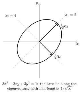Substituting $\mathbf{x} = \mathbf{Q}\mathbf{y}$ , that is, taking $y_i = \langle \mathbf{x}, \mathbf{q}_i \rangle$ to be the coordinates of $\mathbf{x}$ in that basis, $q(\mathbf{x}) = \sum_{i=1}^{n} \lambda_i y_i^2 .$ In particular, for $n = 2$ with $\lambda_1, \lambda_2 > 0$ , the level set $\{q = 1\}$ is an ellipse whose axes lie along $\mathbf{q}_1$ and $\mathbf{q}_2$ , with half-lengths $1/\sqrt{\lambda_1}$ and $1/\sqrt{\lambda_2}$ .

Proof. Since $\mathbf{Q}$ is invertible, $\mathbf{x} = \mathbf{Q}\mathbf{y}$ sets up a bijection between $\mathbf{x}$ and $\mathbf{y} = \mathbf{Q}^{-1}\mathbf{x} = \mathbf{Q}^{\top}\mathbf{x}$ , whose $i$ -th entry is $\mathbf{q}_i^{\top}\mathbf{x} = \langle \mathbf{x}, \mathbf{q}_i \rangle$ . Substituting, $q(\mathbf{Q}\mathbf{y}) = (\mathbf{Q}\mathbf{y})^{\top}\mathbf{A}(\mathbf{Q}\mathbf{y}) = \mathbf{y}^{\top}(\mathbf{Q}^{\top}\mathbf{A}\mathbf{Q})\mathbf{y} = \mathbf{y}^{\top}\mathbf{D}\mathbf{y} = \sum_i \lambda_iy_i^2 ,$ using $(\mathbf{Q}\mathbf{y})^{\top} = \mathbf{y}^{\top}\mathbf{Q}^{\top}$ (Theorem 0.9.5).

For $n = 2$ with both $\lambda_i > 0$ , the condition $q(\mathbf{x}) = 1$ becomes $\lambda_1y_1^2 + \lambda_2y_2^2 = 1$ , the standard equation of an ellipse in the $\mathbf{y}$ coordinates, meeting the $y_1$ -axis where $y_1 = \pm 1/\sqrt{\lambda_1}$ and the $y_2$ -axis where $y_2 = \pm 1/\sqrt{\lambda_2}$ . Those axes are the lines $\operatorname{span}(\mathbf{q}_1)$ and $\operatorname{span}(\mathbf{q}_2)$ of the original picture, because $\mathbf{y} = \mathbf{e}_1$ corresponds to $\mathbf{x} = \mathbf{Q}\mathbf{e}_1 = \mathbf{q}_1$ . Since $\mathbf{Q}$ is orthogonal, it preserves lengths (Theorem 11.7.3), so the half-lengths are unchanged by the substitution.

Example (Finding the axes of a conic)

Identify the curve $3x^2 - 2xy + 3y^2 = 1$ in $\mathbb{R}^2$ , and find its axes and their half-lengths.

Solution. The symmetric matrix of the form is $\mathbf{A} = \begin{pmatrix} 3 & -1 \\ -1 & 3 \end{pmatrix},$ the off-diagonal entries being half of $-2$ . Its characteristic polynomial is $x^2 - 6x + 8$ , so the eigenvalues are $2$ and $4$ . For $\lambda = 2$ , $\mathbf{A} - 2\mathbf{I} = \begin{pmatrix} 1 & -1 \\ -1 & 1 \end{pmatrix}$ gives $x = y$ and the unit eigenvector $\mathbf{q}_1 = \tfrac1{\sqrt2}(1,1)$ . For $\lambda = 4$ , $\mathbf{A} - 4\mathbf{I} = \begin{pmatrix} -1 & -1 \\ -1 & -1 \end{pmatrix}$ gives $x = -y$ and $\mathbf{q}_2 = \tfrac1{\sqrt2}(1,-1)$ .

In the coordinates $y_1 = \langle \mathbf{x}, \mathbf{q}_1 \rangle$ , $y_2 = \langle \mathbf{x}, \mathbf{q}_2 \rangle$ , the equation is $2y_1^2 + 4y_2^2 = 1$ . Both eigenvalues are positive, so the curve is an ellipse. Its major axis lies along $\mathbf{q}_1$ , the line $y = x$ , with half-length $1/\sqrt2$ ; its minor axis lies along $\mathbf{q}_2$ , the line $y = -x$ , with half-length $1/2$ . The check is that $\tfrac1{\sqrt2}(1,1)$ scaled to length $1/\sqrt2$ is the point $(\tfrac12, \tfrac12)$ , and $3\cdot\tfrac14 - 2\cdot\tfrac14 + 3\cdot\tfrac14 = 1$ .

$Diagram. Labels: x, y, tfrac 1sqrt 2q_1, tfrac 12q_2, lambda_1 = 2, lambda_2 = 4, 3x^2-2xy+3y^2=1: the axes lie along the\\ eigenvectors, with half-lengths 1/sqrt lambda_i$

Two features of the picture are worth naming. The axes are orthogonal because the eigenvectors are, and that is the whole content of the theorem; a non-symmetric matrix in the same role would produce a pair of distinguished directions that need not be perpendicular. And the bigger eigenvalue gives the shorter axis, since the half-length is $1/\sqrt{\lambda}$ : a large $\lambda$ makes $q$ reach the value $1$ sooner.

Remark. Chapter 14 will diagonalize quadratic forms again, but by congruence: replacing $\mathbf{A}$ by $\mathbf{P}^{\top}\mathbf{A}\mathbf{P}$ for an arbitrary invertible $\mathbf{P}$ , not necessarily orthogonal. That is a weaker relation, and it destroys the eigenvalues while preserving only their signs, which is Sylvester’s law of inertia. What makes the present theorem special is that $\mathbf{Q}^{\top} = \mathbf{Q}^{-1}$ , so $\mathbf{Q}^{\top}\mathbf{A}\mathbf{Q} = \mathbf{Q}^{-1}\mathbf{A}\mathbf{Q}$ and the two relations coincide: an orthogonal change of variables is a similarity and a congruence, so it keeps the eigenvalues and the geometry at once.

Warning. The theorem needs $\mathbb{R}$ , and symmetry is not the same as having real eigenvalues. The matrix $\begin{pmatrix} 1 & 1 \\ 1 & 0 \end{pmatrix}$ is symmetric with rational entries, but its eigenvalues are $(1 \pm \sqrt5)/2$ , which are irrational; over $\mathbb{Q}$ there is no eigenvector at all, and no version of Theorem 12.5.1 survives. Conversely $\begin{pmatrix} 1 & 1 \\ 0 & 2 \end{pmatrix}$ has the real eigenvalues $1$ and $2$ and is not symmetric; real eigenvalues alone buy nothing, since they do not make the eigenvectors orthogonal.

12.5.6. Exercises

A. Check your understanding

Exercise (A1)

(a) State the real spectral theorem and its matrix form, with every hypothesis.
(b) Which two results from Section 2 does the induction use, and what does each one supply?
(c) True or false: a normal operator on a real inner product space has an orthonormal basis of eigenvectors. Justify your answer.
(d) What are the possible diagonal blocks in the real normal form of a normal operator, and what does the condition $b > 0$ rule out?
(e) Given a symmetric $\mathbf{A}$ with orthonormal eigenvectors $\mathbf{q}_1, \mathbf{q}_2$ and eigenvalues $9$ and $1$ , describe the curve $\mathbf{x}^{\top}\mathbf{A}\mathbf{x} = 1$ .
(f) True or false: a real matrix with real eigenvalues is symmetric. Justify your answer.

Solution.

(a) For a finite-dimensional real inner product space $V$ and $T \in \mathcal{L}(V)$ : $T$ is self-adjoint if and only if $V$ has an orthonormal basis of eigenvectors (Theorem 12.5.1). Matrix form: $\mathbf{A} \in M_n(\mathbb{R})$ is symmetric if and only if $\mathbf{A} = \mathbf{Q}\mathbf{D}\mathbf{Q}^{\top}$ with $\mathbf{Q}$ orthogonal and $\mathbf{D}$ real diagonal (Corollary 12.5.2).
(b) Theorem 12.2.2 supplies one eigenvector to peel off, and Theorem 12.2.4 supplies the smaller object to induct on, namely the self-adjoint restriction to the orthogonal complement.
(c) False. The quarter turn of $\mathbb{R}^2$ is normal and has no eigenvector at all (Example (A normal real operator with no eigenvector)).
(d) Blocks $(c)$ with $c \in \mathbb{R}$ , and $2 \times 2$ blocks $\boldsymbol{\Lambda}(\lambda) = \begin{pmatrix} a & -b \\ b & a \end{pmatrix}$ with $b > 0$ (Theorem 12.5.3). The condition $b > 0$ rules out the transposed block $\boldsymbol{\Lambda}(\conj\lambda)$ , which is orthogonally similar to it via $\operatorname{diag}(1, -1)$ ; fixing the sign is what makes the list of blocks well defined.
(e) An ellipse with axes along $\mathbf{q}_1$ and $\mathbf{q}_2$ , of half-lengths $1/3$ and $1$ (Theorem 12.5.5). The longer axis is along $\mathbf{q}_2$ , the eigenvector for the smaller eigenvalue.
(f) False. $\begin{pmatrix} 1 & 1 \\ 0 & 2 \end{pmatrix}$ has eigenvalues $1, 2$ and is not symmetric. The correct statement is the converse: a symmetric real matrix has real eigenvalues.

B. Practice

Exercise (B1: Orthogonally diagonalize)

For each symmetric matrix, find an orthogonal $\mathbf{Q}$ and a diagonal $\mathbf{D}$ with $\mathbf{Q}^{\top}\mathbf{A}\mathbf{Q} = \mathbf{D}$ .

(a) $\mathbf{A} = \begin{pmatrix} 1 & 2 \\ 2 & 1 \end{pmatrix}$ .
(b) $\mathbf{A} = \begin{pmatrix} 4 & 0 & 1 \\ 0 & 2 & 0 \\ 1 & 0 & 4 \end{pmatrix}$ .

Solution.

(a) $p_{\mathbf{A}}(x) = x^2 - 2x - 3 = (x-3)(x+1)$ , so the eigenvalues are $3$ and $-1$ . For $\lambda = 3$ , $\mathbf{A} - 3\mathbf{I} = \begin{pmatrix} -2 & 2 \\ 2 & -2 \end{pmatrix}$ gives $x_1 = x_2$ and $\mathbf{q}_1 = \tfrac1{\sqrt2}(1,1)$ ; for $\lambda = -1$ , $\mathbf{q}_2 = \tfrac1{\sqrt2}(1,-1)$ . Hence $\mathbf{Q} = \tfrac1{\sqrt2}\begin{pmatrix} 1 & 1 \\ 1 & -1 \end{pmatrix}, \qquad \mathbf{D} = \begin{pmatrix} 3 & 0 \\ 0 & -1 \end{pmatrix} .$
(b) The second coordinate is untouched: $\mathbf{A}\mathbf{e}_2 = 2\mathbf{e}_2$ . On $\operatorname{span}(\mathbf{e}_1, \mathbf{e}_3)$ the matrix acts as $\begin{pmatrix} 4 & 1 \\ 1 & 4 \end{pmatrix}$ , with eigenvalues $5$ and $3$ and eigenvectors $(1,1)$ and $(1,-1)$ there. Lifting back, $\mathbf{q}_1 = \tfrac1{\sqrt2}(1,0,1), \quad \mathbf{q}_2 = \tfrac1{\sqrt2}(-1,0,1), \quad \mathbf{q}_3 = (0,1,0),$ with eigenvalues $5, 3, 2$ . These are orthonormal, so $\mathbf{Q} = (\mathbf{q}_1 \mid \mathbf{q}_2 \mid \mathbf{q}_3)$ is orthogonal and $\mathbf{Q}^{\top}\mathbf{A}\mathbf{Q} = \operatorname{diag}(5, 3, 2)$ . As a check, $5 + 3 + 2 = 10 = \operatorname{tr} \mathbf{A}$ .

Exercise (B2: Identify the conic)

Identify the curve $5x^2 + 4xy + 5y^2 = 1$ : say what kind of conic it is, find its axes, and find their half-lengths.

Solution. The symmetric matrix of the form is $\mathbf{A} = \begin{pmatrix} 5 & 2 \\ 2 & 5 \end{pmatrix}$ , the off-diagonal entries being half of $4$ . Its characteristic polynomial is $x^2 - 10x + 21 = (x-7)(x-3)$ , so the eigenvalues are $7$ and $3$ . For $\lambda = 7$ , $\mathbf{A} - 7\mathbf{I} = \begin{pmatrix} -2 & 2 \\ 2 & -2 \end{pmatrix}$ gives $\mathbf{q}_1 = \tfrac1{\sqrt2}(1,1)$ ; for $\lambda = 3$ , $\mathbf{q}_2 = \tfrac1{\sqrt2}(1,-1)$ .

By Theorem 12.5.5 the equation becomes $7y_1^2 + 3y_2^2 = 1$ . Both eigenvalues are positive, so the curve is an ellipse. Its axes are the lines $y = x$ and $y = -x$ , with half-lengths $1/\sqrt7$ along $\mathbf{q}_1$ and $1/\sqrt3$ along $\mathbf{q}_2$ ; the major axis is the second one. Check: the point $\tfrac1{\sqrt3}\mathbf{q}_2 = \tfrac1{\sqrt6}(1,-1)$ gives $\tfrac56 - \tfrac46 + \tfrac56 = 1$ .

Exercise (B3: A sum of rank-one projections)

Using your answer to Exercise (B1: Orthogonally diagonalize) (b), write $\mathbf{A} = \begin{pmatrix} 4 & 0 & 1 \\ 0 & 2 & 0 \\ 1 & 0 & 4 \end{pmatrix}$ as $\sum_i \lambda_i\mathbf{q}_i\mathbf{q}_i^{\top}$ , with the three matrices $\mathbf{q}_i\mathbf{q}_i^{\top}$ written out, and verify the identity by adding them.

Solution. With $\mathbf{q}_1 = \tfrac1{\sqrt2}(1,0,1)$ , $\mathbf{q}_2 = \tfrac1{\sqrt2}(-1,0,1)$ , $\mathbf{q}_3 = (0,1,0)$ and $\lambda = 5, 3, 2$ , $\mathbf{q}_1\mathbf{q}_1^{\top} = \tfrac12\begin{pmatrix} 1 & 0 & 1 \\ 0 & 0 & 0 \\ 1 & 0 & 1 \end{pmatrix}, \qquad \mathbf{q}_2\mathbf{q}_2^{\top} = \tfrac12\begin{pmatrix} 1 & 0 & -1 \\ 0 & 0 & 0 \\ -1 & 0 & 1 \end{pmatrix},$ and $\mathbf{q}_3\mathbf{q}_3^{\top}$ is the matrix with a single $1$ in position $(2,2)$ . Then $5\,\mathbf{q}_1\mathbf{q}_1^{\top} + 3\,\mathbf{q}_2\mathbf{q}_2^{\top} = \begin{pmatrix} 4 & 0 & 1 \\ 0 & 0 & 0 \\ 1 & 0 & 4 \end{pmatrix},$ since $\tfrac12(5+3) = 4$ on the diagonal and $\tfrac12(5-3) = 1$ off it. Adding $2\,\mathbf{q}_3\mathbf{q}_3^{\top}$ inserts the $2$ in position $(2,2)$ and gives $\mathbf{A}$ , as Corollary 12.5.4 requires.

C. Going deeper

Exercise (C1: One eigenvalue only)

(a) Let $\mathbf{A} \in M_n(\mathbb{R})$ be symmetric with every eigenvalue equal to $\lambda$ . Prove that $\mathbf{A} = \lambda\mathbf{I}$ .
(b) Show that (a) fails without symmetry, by exhibiting a matrix in $M_2(\mathbb{R})$ whose only eigenvalue is $0$ and which is not $\mathbf{0}$ .
(c) Deduce that a symmetric $\mathbf{A}$ with $\mathbf{A}^2 = \mathbf{A}$ is the matrix of an orthogonal projection.

Solution.

(a) By Corollary 12.5.2, $\mathbf{A} = \mathbf{Q}\mathbf{D}\mathbf{Q}^{\top}$ with $\mathbf{D}$ diagonal carrying the eigenvalues, so $\mathbf{D} = \lambda\mathbf{I}$ . Hence $\mathbf{A} = \mathbf{Q}(\lambda\mathbf{I})\mathbf{Q}^{\top} = \lambda\mathbf{Q}\mathbf{Q}^{\top} = \lambda\mathbf{I}$ .
(b) $\mathbf{J}_2(0) = \begin{pmatrix} 0 & 1 \\ 0 & 0 \end{pmatrix}$ has characteristic polynomial $x^2$ , so $0$ is its only eigenvalue, and it is not the zero matrix. It is of course not symmetric.
(c) If $\mathbf{A}^2 = \mathbf{A}$ and $\mathbf{A}\mathbf{x} = \lambda\mathbf{x}$ with $\mathbf{x} \neq \mathbf{0}$ , then $\lambda^2\mathbf{x} = \mathbf{A}^2\mathbf{x} = \mathbf{A}\mathbf{x} = \lambda\mathbf{x}$ , so $\lambda^2 = \lambda$ and $\lambda \in \{0, 1\}$ . By Corollary 12.5.2, $\mathbf{A} = \mathbf{Q}\mathbf{D}\mathbf{Q}^{\top}$ with $\mathbf{D}$ diagonal of zeros and ones, so $\mathbf{A} = \sum_{i \in S}\mathbf{q}_i\mathbf{q}_i^{\top}$ where $S$ indexes the eigenvalue $1$ (Corollary 12.5.4). That is the sum of the projections onto an orthonormal basis of $U = E_1(\mathbf{A})$ , which is the orthogonal projection $P_U$ by Theorem 11.3.3.

Exercise (C2: Diagonalizing two matrices at once)

Let $\mathbf{A}, \mathbf{B} \in M_n(\mathbb{R})$ be symmetric with $\mathbf{A}\mathbf{B} = \mathbf{B}\mathbf{A}$ .

(a) Prove that each eigenspace $E_{\lambda}(\mathbf{A})$ is $\mathbf{B}$ -invariant, and that the restriction of $T_{\mathbf{B}}$ to it is self-adjoint.
(b) Prove that there is a single $\mathbf{Q} \in \operatorname{O}(n)$ with $\mathbf{Q}^{\top}\mathbf{A}\mathbf{Q}$ and $\mathbf{Q}^{\top}\mathbf{B}\mathbf{Q}$ both diagonal.
(c) Show that the conclusion fails without commutativity, using $\begin{pmatrix} 1 & 0 \\ 0 & 0 \end{pmatrix}$ and $\begin{pmatrix} 0 & 1 \\ 1 & 0 \end{pmatrix}$ .

Hint for (b): apply Theorem 12.5.1 inside each eigenspace of $\mathbf{A}$ .

Solution.

(a) Invariance is Theorem 9.9.1: if $\mathbf{A}\mathbf{x} = \lambda\mathbf{x}$ then $\mathbf{A}(\mathbf{B}\mathbf{x}) = \mathbf{B}(\mathbf{A}\mathbf{x}) = \lambda\mathbf{B}\mathbf{x}$ . For self-adjointness of the restriction, take $\mathbf{u}, \mathbf{v} \in E_{\lambda}(\mathbf{A})$ ; then $\langle \mathbf{B}\mathbf{u}, \mathbf{v} \rangle = \langle \mathbf{u}, \mathbf{B}\mathbf{v} \rangle$ because $\mathbf{B}$ is symmetric on all of $\mathbb{R}^n$ , and both $\mathbf{B}\mathbf{u}$ and $\mathbf{B}\mathbf{v}$ lie in $E_{\lambda}(\mathbf{A})$ by the first part, so the identity holds inside the subspace with its restricted inner product.
(b) Let $\lambda_1, \dots, \lambda_k$ be the distinct eigenvalues of $\mathbf{A}$ . By Theorem 12.5.1, $\mathbb{R}^n$ is the direct sum of the eigenspaces $E_{\lambda_i}(\mathbf{A})$ , and these are mutually orthogonal (Theorem 12.2.3). By (a) and Theorem 12.5.1 applied to the self-adjoint operator $T_{\mathbf{B}}|_{E_{\lambda_i}(\mathbf{A})}$ , each $E_{\lambda_i}(\mathbf{A})$ has an orthonormal basis of eigenvectors of $\mathbf{B}$ . Every vector of $E_{\lambda_i}(\mathbf{A})$ is an eigenvector of $\mathbf{A}$ , so these basis vectors are common eigenvectors. Stringing the $k$ bases together gives an orthonormal basis of $\mathbb{R}^n$ , orthonormal across the blocks because distinct eigenspaces of $\mathbf{A}$ are orthogonal. Let $\mathbf{Q}$ have those vectors as columns; then $\mathbf{Q} \in \operatorname{O}(n)$ and both $\mathbf{Q}^{\top}\mathbf{A}\mathbf{Q}$ and $\mathbf{Q}^{\top}\mathbf{B}\mathbf{Q}$ are diagonal.
(c) These two do not commute: $\mathbf{A}\mathbf{B} = \begin{pmatrix} 0 & 1 \\ 0 & 0 \end{pmatrix}$ while $\mathbf{B}\mathbf{A} = \begin{pmatrix} 0 & 0 \\ 1 & 0 \end{pmatrix}$ . And no common eigenbasis exists: the eigenvectors of $\mathbf{A}$ are the multiples of $\mathbf{e}_1$ and of $\mathbf{e}_2$ , while $\mathbf{B}\mathbf{e}_1 = \mathbf{e}_2$ is not a multiple of $\mathbf{e}_1$ . Commutativity is necessary as well as sufficient, since two simultaneously diagonalized matrices commute.

Exercise (C3: A rotation-scaling in normal form)

Let $\mathbf{A} = \begin{pmatrix} 3 & 4 \\ -4 & 3 \end{pmatrix} \in M_2(\mathbb{R})$ .

(a) Verify that $\mathbf{A}$ is normal and not symmetric, and find its complex eigenvalues.
(b) Find an orthogonal $\mathbf{Q}$ with $\mathbf{Q}^{\top}\mathbf{A}\mathbf{Q} = \boldsymbol{\Lambda}(\lambda)$ for the eigenvalue $\lambda$ with positive imaginary part.
(c) Explain why no orthogonal $\mathbf{Q}$ makes $\mathbf{Q}^{\top}\mathbf{A}\mathbf{Q}$ diagonal, and why this does not contradict Theorem 12.4.2.

Solution.

(a) $\mathbf{A}^{\top}\mathbf{A} = \mathbf{A}\mathbf{A}^{\top} = 25\mathbf{I}$ , so $\mathbf{A}$ is normal; $\mathbf{A}^{\top} \neq \mathbf{A}$ since $4 \neq -4$ . Its characteristic polynomial is $x^2 - 6x + 25 = (x-3)^2 + 16$ , with roots $3 \pm 4i$ .
(b) The eigenvalue with positive imaginary part is $\lambda = 3 + 4i$ , so $\boldsymbol{\Lambda}(\lambda) = \begin{pmatrix} 3 & -4 \\ 4 & 3 \end{pmatrix}$ . Take $\mathbf{Q} = \operatorname{diag}(1, -1)$ , which is orthogonal. Then $\mathbf{Q}^{\top}\mathbf{A}\mathbf{Q} = \begin{pmatrix} 1 & 0 \\ 0 & -1 \end{pmatrix} \begin{pmatrix} 3 & 4 \\ -4 & 3 \end{pmatrix} \begin{pmatrix} 1 & 0 \\ 0 & -1 \end{pmatrix} = \begin{pmatrix} 3 & -4 \\ 4 & 3 \end{pmatrix},$ which is $\boldsymbol{\Lambda}(3 + 4i)$ . This is Case 2 of the proof of Theorem 12.5.3 with $p = 3$ and $q = 4$ .
(c) If $\mathbf{Q}^{\top}\mathbf{A}\mathbf{Q}$ were diagonal for some $\mathbf{Q} \in \operatorname{O}(2)$ , then $\mathbf{A} = \mathbf{Q}\mathbf{D}\mathbf{Q}^{\top}$ would be symmetric by Corollary 12.5.2, and it is not. There is no contradiction with Theorem 12.4.2, which concerns a complex inner product space: over $\mathbb{C}^2$ the matrix $\mathbf{A}$ is indeed unitarily diagonalizable, to $\operatorname{diag}(3+4i, 3-4i)$ , but the diagonalizing basis $\tfrac1{\sqrt2}(1, \pm i)$ is not real, so it is unavailable inside $\mathbb{R}^2$ .